Chapter 11 Chi-Squared

Figure 11.1: A Statypus Has Graduated to Advanced Statistics

A platypus has approximately 40,000 electric sensors in their bills which they use to locate invertebrates which are buried in riverbeds. This extra “sense” is called electroreception.¹⁸⁰

The Normal Distribution has proven quite fruitful in our investigation of symmetric and unimodal data, especially with the addition of Student’s \(t\)-Distributions. However, it is not well suited for skewed data or data that cannot be negative. For example, if we are trying to understand a population standard deviation or variance, then we need a distribution that has 0 probability for values less than 0. The \(\chi^2\) Distribution¹⁸¹ will serve this purpose and more. It will also be a valuable tool for investigating categorical data.

New R Functions Used

All functions listed below have a help file built into RStudio. Most of these functions have options which are not fully covered or not mentioned in this chapter. To access more information about other functionality and uses for these functions, use the ? command. E.g. To see the help file for qnorm, you can run ?pchisq or ?pchisq() in either an R Script or in your Console.

We will see the following functions in Chapter 11.

• round(): Rounds the value to the specified number of decimal places (default 0).

• pchisq(): Distribution function for the \(\chi^2\) distribution.

• chisq.test(): Performs chi-squared contingency table tests and goodness-of-fit tests.

• as.matrix(): Attempts to turn its argument into a matrix.

• addmargins(): Adds Sum values to a table.

• marginSums(): Computes the row or column totals of a table.

• M %*% N: The operation M %*% N does the matrix multiplication of M and N.

To load all of the datasets used in Chapter 11, run the following line of code.

load(url("https://statypus.org/files/StatypusCh11.RData"))

11.1 The Chi-Squared Distribution

If we were to look at a collection of random \(z\) values, i.e. pull a sample from \(\text{Norm}(0,1)\), then we expect the resulting distribution to be modeled by the Standard Normal Distribution. Below is a histogram of 100,000 random values from \(\text{Norm}(0,1)\) as well as the Standard Normal Distribution superimposed on it.

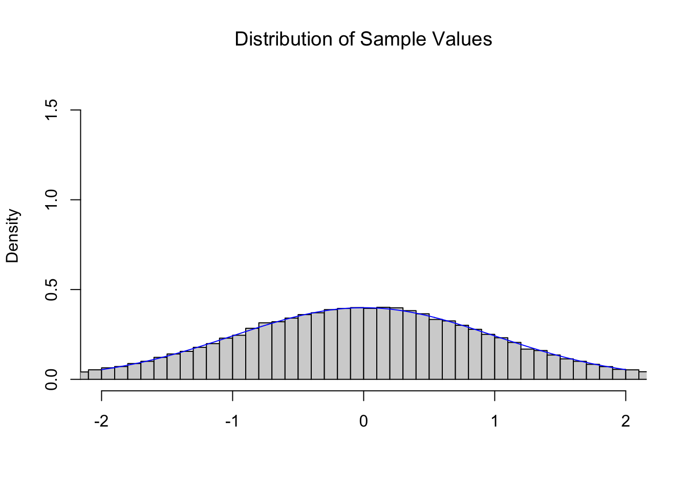
Figure 11.2: Illustration of the Central Limit Theorem

As expected, random \(z\) values follow the \(z\) distribution, the Standard Normal Distribution.

We have intentionally used a somewhat awkward graphing window for the histogram, but this is so that we can use the same graphing window for all of the graphs in this section.

The Central Limit Theorem (CLT), Theorem 9.1, tells us that if we repeatedly find the mean of 4 random values from the Standard Normal Distribution we get another Normal distribution with a mean of \(0\) and a standard deviation of \(\frac{\sigma_x}{\sqrt{n}} = \frac{1}{\sqrt{4}} = \frac{1}{2}\). Below is the histogram of 100,000 sample means of size \(n=4\) from the Standard Normal Distribution and the theoretical distribution \(\text{Norm}\left(0,\frac{1}{2}\right)\).

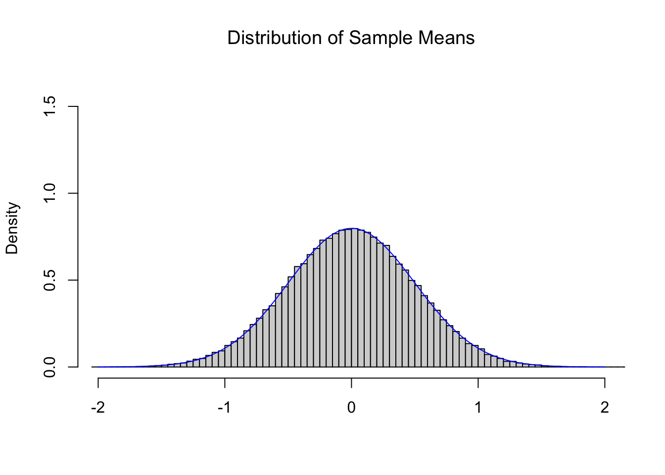
Figure 11.3: Illustration of the Central Limit Theorem

Comparing this to Figure 11.2, we see a distribution which is narrowing, but maintains a center near 0. The CLT also tells us that as we increase the value of \(n\) that we get tighter and tighter distributions such as the one below for \(n = 16\).

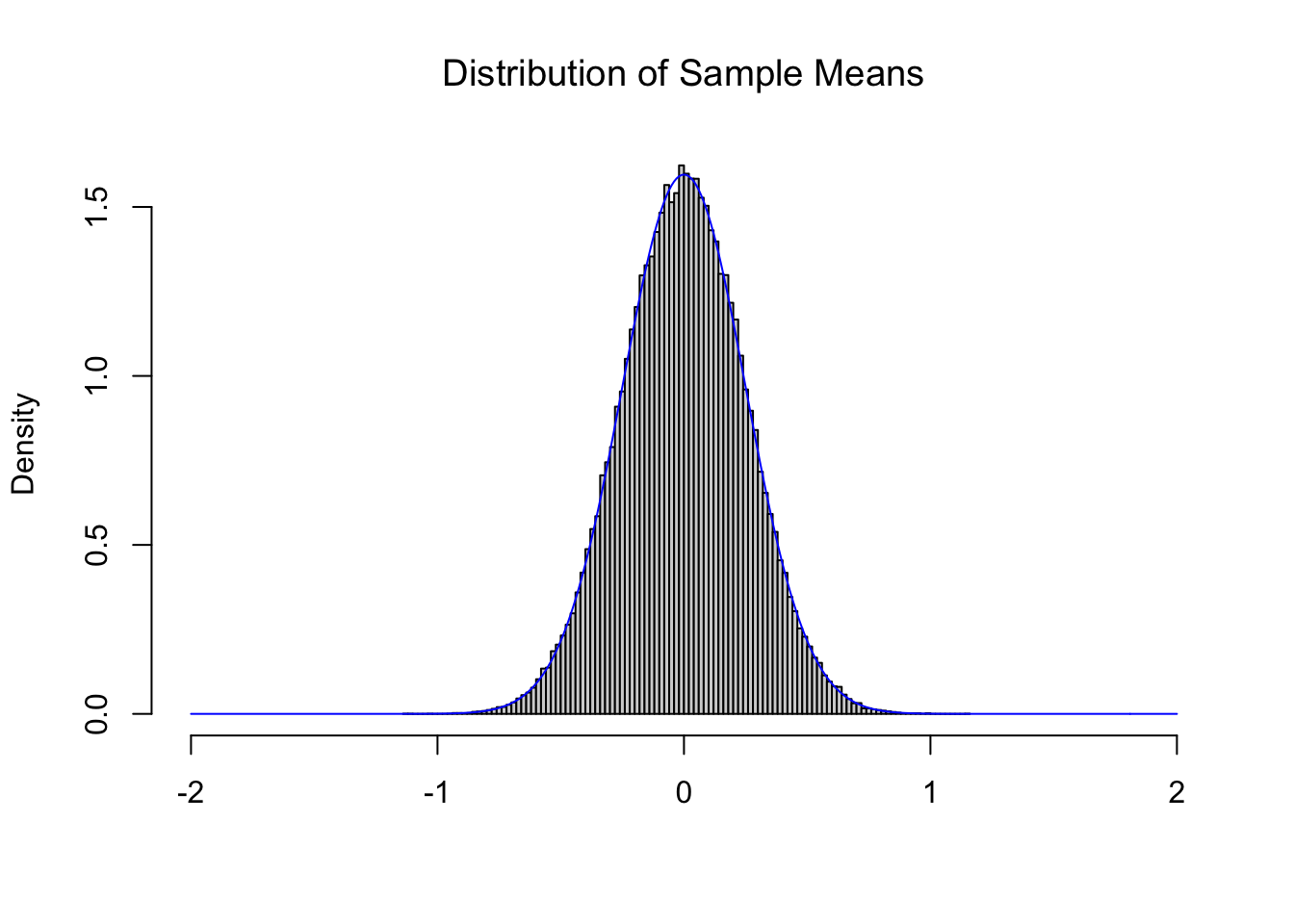
Figure 11.4: Illustration of the Central Limit Theorem

Tying it all together, below is the theoretical distributions \(\text{Norm}\left( 0, \frac{1}{\sqrt{n}}\right)\) for \(n = 1, 2, 3, \ldots, 16\).

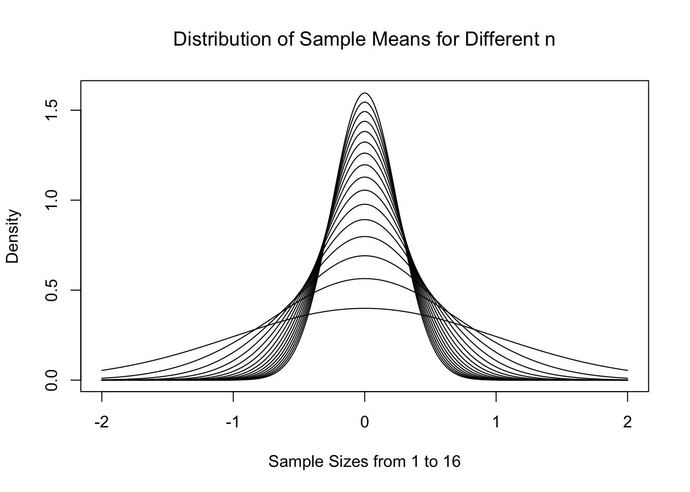
Figure 11.5: Central Limit Theorem for Increasing \(n\)

As expected, the distributions start to centralize on the limit of \(\mu_{\bar{x}} = \mu = 0\). This is all work we heavily leveraged in Chapter 10 to do inference on a population mean. However, what if we wanted to model something other than the sample mean?

11.1.1 A Model for (Scaled) Variances

We have been sampling from \(\text{Norm}(0,1)\) by selecting numerous samples of size \(n\). At the beginning of Section 11.1, we looked at the distributions of values of \(\bar{x}\) for fixed values of \(n\) and realized that the CLT told us the exact distribution that would model that statistic. Being that we were sampling from \(\text{Norm}(0,1)\), we found that \(\bar{x}\) were estimates of \(\mu = 0\).

However, if we were to look at values of \(s\), they should be an estimate of \(\sigma = 1\). For slightly technical reasons, we will really want to consider the sample variance, or the sample standard deviation squared (\(s^2\)), which should be an estimate of the population variance which is \(\sigma^2 = 1^2 = 1\). If we calculated the sample variance¹⁸² of our 100,000 samples of size \(n=4\), we get the following distribution.

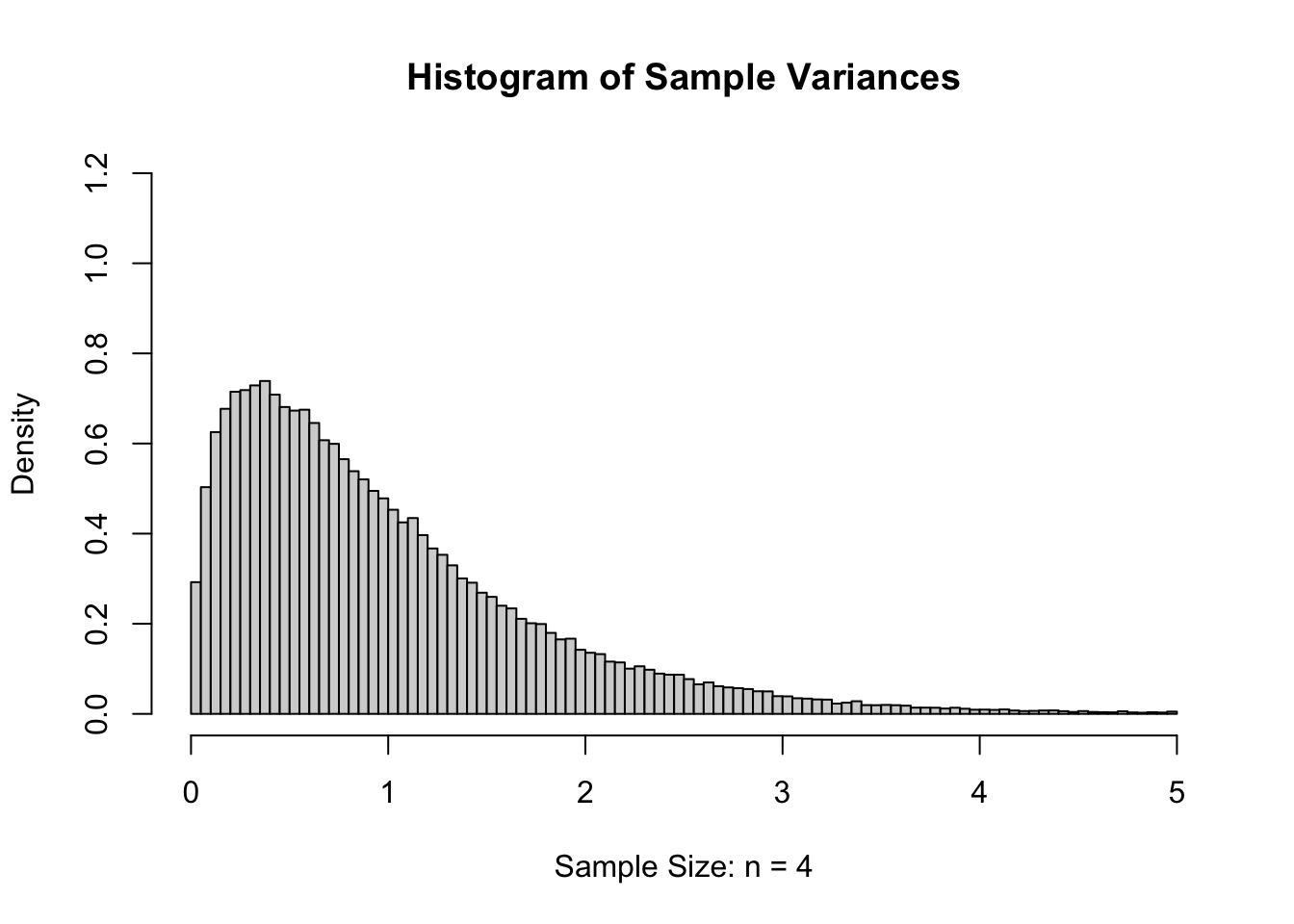
Figure 11.6: Sample Variances for \(n=4\)

If we again increase \(n\) to 16 and again give the histogram of the sample variances, we get the following.

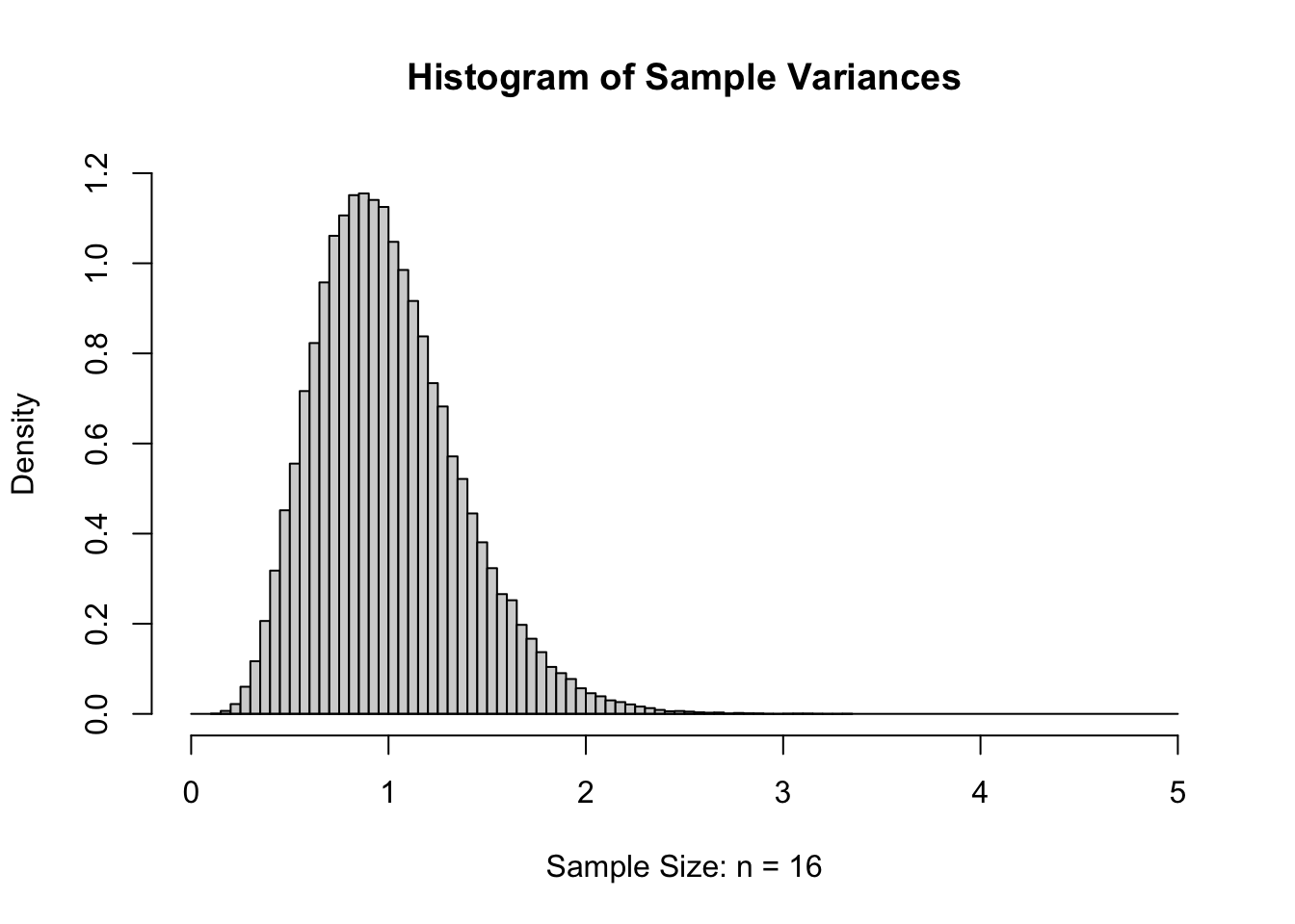
Figure 11.7: Sample Variances for \(n=16\)

While the formulas are well beyond the scope of this document, below is the collection of theoretical distributions that the sample variances should follow. We remind the reader that for a sample of size \(n\), that we say that the degrees of freedom, or \(\nu\) (as in Definition 4.8 or Definition 10.3), is \(n-1\). So if \(n\) is between 4 and 16 then \(\nu\) is between 3 and 15.

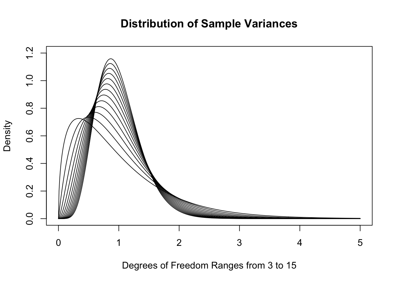
Figure 11.8: Sample Variances for \(n=4, 5,..., 16\)

As \(n\) increases, the distributions do get much denser near 1. In fact, the skew also decreases as \(n\) increases. While we very well could use these distributions in our investigation¹⁸³, the traditional method is to look at the distribution of sample variances multiplied by the degrees of freedom. We will call these the scaled sample variances.

Definition 11.1 Given a vector \({\bf x} = ( x_1, x_2, \ldots, x_n )\) having \(n\) values (with \(n\geq 2\)), we define the Scaled Sample Variance, denoted \(\text{SSV}\), to be the product of the Sample Variance and the Degrees of Freedom (See Definition 4.8).

\[\text{SSV} = (n-1)\cdot s ^2 = \sum (x - \bar{x})^2\]

The above definition points out that we are actually simply looking at the sum of the squares of the \(n\) deviations.¹⁸⁴ This is what we called SumSquareDevx in Chapter 4. That is to say we are considering a model for either the scaled sample variances or the sum of the squared deviations. As the distributions in Figure 11.8 have maxima which are near 1, the result of multiplying by \(\nu\) is to place the maxima near \(n-1\) for samples of size \(n\). Below is a plot of these theoretical distributions.

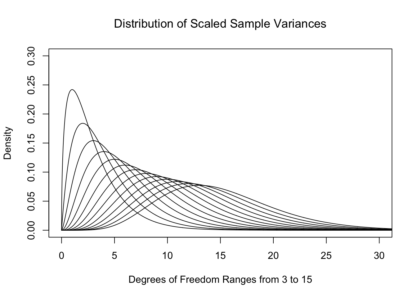
Figure 11.9: Plot of Chi Squared for Different Degrees of Freedom

That is to say, just like for Student’s \(t\)-Distribution, we get a different distribution for each value of the degrees of freedom, \(\nu\). We call these new distributions the \(\chi^2\) Distributions.

Definition 11.2 For any positive integer \(\nu\), the \(\chi^2\) Distribution with \(\nu\) Degrees of Freedom is the distribution of the scaled sample variances of samples of size \(n = \nu + 1\) from \(\text{Norm}(0,1)\).

While we have only defined the \(\chi^2\) distribution for positive integer values of \(\nu\), there are actually distributions for any positive real value of \(\nu\). In addition, the equation \(n = \nu + 1\) is equivalent to the equation \(\nu = n -1\) which we previously used in Chapters 4 and 10.

While we have defined the \(\chi^2\) distribution as a model of scaled sample variances, we will actually use it for alternate analyses in Sections 11.2 and 11.4.

It may be curious if the histogram of the sum the squares of \(n\) deviations should be modeled by \(\chi^2\) with \(n\) or \(n-1\) degrees of freedom since the \(n-1\) term no longer exists. To inspect this, we go back to our 100,000 samples of size \(n=4\) and plot the scaled sample variances below. We see that \(\nu=3\) much more closely resembles our samples than using \(\nu = 4\). (For technical reasons, we use df in lieu of \(\nu\) in the titles of the plot below for the degrees of freedom.)

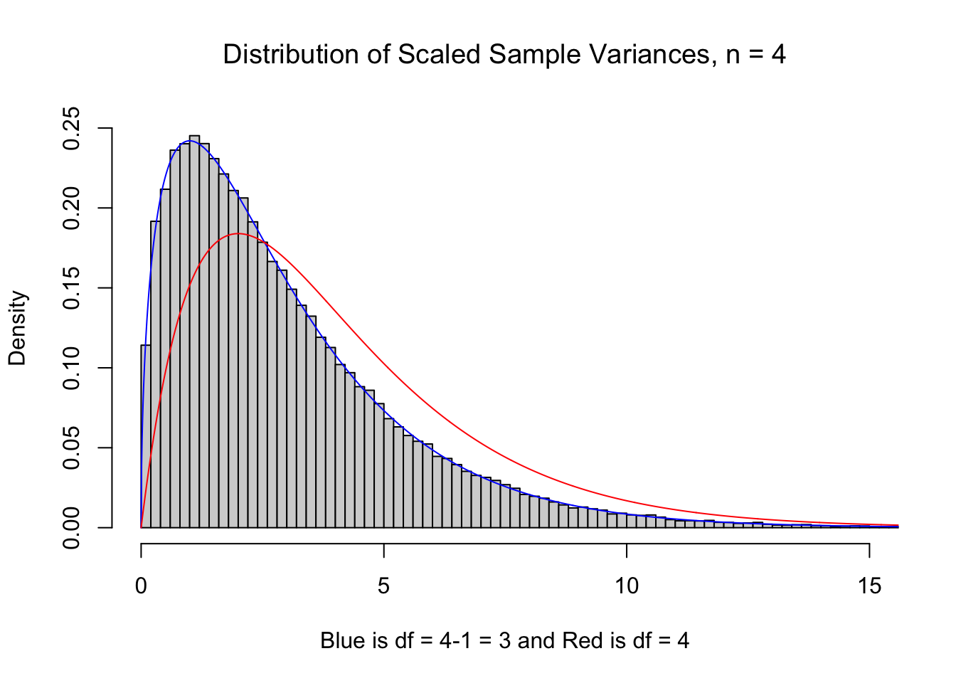
Figure 11.10: df = n vs. df = n-1

11.1.2 Defining \(X^2\)

We can also define a statistic denoted \(X^2\) for tabulated data that is modeled by the \(\chi^2\) distribution. This will allow us to apply this new model to qualitative variables. For example, we will look at how many individuals in a distributions fall into a collection of categories in Section 11.2 and also look at two-way tables in Section 11.4. Here we give a definition for a way to calculate another statistic that is modeled by the \(\chi^2\) distribution that will work for both of those sections.

Definition 11.3 Given a table of values pulled from a sample, we call the cells of the table the Observed Value of the Cell and will denote them as \(\text{Obs}\) in our calculations. We define the \({\bf \chi^2 }\)-statistic, denoted by \(X^2\), to be given by

\[ X^2 = \sum_{\text{all cells}} \frac{\left(\text{Obs} - \text{Exp}\right)^2}{\text{Exp}} \] where we define the Expected Value of the Cell, denoted as \(\text{Exp}\), to be

\[ \text{Exp} = P(\text{cell})\cdot n \] where \(P(\text{cell})\) is the probability of a random value satisfying the conditions of that cell under the assumed conditions.

Each summand of \(X^2\), i.e. a term of form \(\frac{\left(\text{Obs} - \text{Exp}\right)^2}{\text{Exp}}\), is called an \(\bf X^2\)-Contribution.

The way we find \(P(\text{cell})\) will be dependent on the type of test we are conducting and the associated assumed conditions, and we will define those in the Sections 11.2 and 11.4.

Like we have seen a few times now, parameters often use fancy Greek letters, such as \(\chi^2\), while their associated statistic often use similar Roman (your standard ABCs), such as \(X^2\). So far we have seen the following combinations:

\[\begin{align*} \textbf{S}\text{ample} &\approx \textbf{P}\text{opulation}\\ \textbf{S}\text{tatistic} &\approx \textbf{P}\text{arameter}\\ \textbf{S}\text{ort of } &\approx \textbf{P}\text{erfect}\\ \bar{x} &\approx \mu\\ s &\approx \sigma\\ \text{SE} &\approx \sigma_{\hat{p}} \text{ or } \sigma_{\bar{x}}\\ X^2 &\approx \chi^2 \end{align*}\]

11.2 Chi Squared for Proportions

We can use the \(\chi^2\) distribution to perform new types of hypothesis tests. One example is when if we want to test if a sample comes from a population which is broken into \(N\) different disjoint categories with known proportions. We can calculate the sample proportions of each category, which we call \(\widehat{p_k}\) for \({k = 1, 2, \ldots, N}\), and use them to test if the population proportions for each category, which we call \(p_k\), is equal to a hypothesized value, which we call \(\overline{p_k}\).

In general, a hypothesis test is of form below.

\[ \begin{array}{c|c} H_0 : \text{True Parameter} = \text{Assumed Parameter} &\text{Assumed Situation}\\ H_a : \text{True Parameter} \; \Box \;\text{Assumed Parameter} &\text{Claim Being Tested} \end{array} \] where \(\Box\) is chosen so that \(\text{Sample Statistic} \; \Box \; \text{Assumed Parameter}\) is true.

Definition 11.4 \(\chi^2\)-Test for Proportions Given a sample of \(n\) individuals broken into \(N\) different disjoint categories such that the count of the first category is \(x_1\), the count of the second category is \(x_2\), and so on. This implies that \(x_1 + x_2 + \cdots x_N = n\) and we can further define \(\widehat{p_k} = \frac{x_k}{n}\) so that \(\widehat{p_1} + \widehat{p_2} + \cdots \widehat{p_N} = 1.\)

The following gives an overview of the different proportions we have under consideration.

\[\begin{align*} p_k &= \text{True Population Proportion for category $k$ (True Parameter)}\\ \widehat{p_k} &= \frac{x_k}{n} = \text{Observed Sample Proportion for category $k$ (Statistic)}\\ \overline{p_k} &= \text{Assumed Population Proportion for category $k$ for $H_0$ (Assumed Parameter)} \end{align*}\]

Each of the \(N\) categories gives us a Cell and we say the values of \(x_k\) are the Observed Values, which we denoted \(\text{Obs}\) earlier. We can then define \(P(\text{Cell}) = \overline{p_k}\) for each \(k = 1, 2, \ldots N\). This gives that the Expected Values, which we denoted \(\text{Exp}\) earlier, are the values of \(\overline{p_k}\cdot n\) for all the values of \(k\).

This gives us hypotheses as below.

Theorem 11.1 Given the hypothesis test with the setup of Definition 11.4 as shown below, \[\begin{align*} H_0 :&\; p_1 = \overline{p_1}\\ &\; p_2 = \overline{p_2}\\ &\; \vdots\\ &\; p_n = \overline{p_n}\\ H_a :&\; \text{At least one of the above statements is false,} \end{align*}\] the associated \(p\)-value is the area under the \(\chi^2\) distribution with \(n-1\) degrees of freedom for the values greater than the \(X^2\) statistic as defined in Definition 11.3.

In Theorem 11.1, it is required that \(p_1 + p_2 + \cdots + p_n = 1\). If not, we cannot use the methods here and would need to use prop.test(). See Section 9.6, in particular Example 9.34, for more information.

The above note also gives more motivation for using \(n-1\) degrees of freedom, because the last proportion, \(p_n\), is required to be \(p_n = 1 - p_1 - p_2 - \cdots - p_{n-1}\). That is, we really are only allowed to set \(n-1\) of the \(n\) different \(p_k\) values. The same is true for the \(\overline{p_k}\) values.

When running a \(\chi^2\)-test of Proportions:

• the assumption, \(H_0\), is that our data agrees with the assumed proportions
• the claim, \(H_a\), is that our data does not agree with the assumed proportions

If the \(p\)-value falls at or below the level of significance, \(\alpha\), then we can reject our assumption and state that we have sufficient evidence (at this level of significance) to conclude that the claim, \(H_a\) is true.

If the \(p\)-value is greater than \(\alpha\), then we have insufficient evidence to abandon the assumption contained in \(H_0\).

It is likely that this is still a bit confusing, so we will explain this type of hypothesis test via an example involving \(\text{M}\&\text{M}\)s.

Example 11.1 (M and Ms by Factory: Part 1) Imagine that we find 2 bags of \(\text{M}\&\text{M}\)s, each of which weighs 1 pound, which we will call Bag A and Bag B. We open the bags and break the \(\text{M}\&\text{M}\)s into groups based on their color. We find that Bag A has the following colors

##    Red Orange Yellow  Green   Blue  Brown 
##     59    119     75     60    126     69

and Bag B is as follows.

##    Red Orange Yellow  Green   Blue  Brown 
##     62     95     76    114    107     70

We are going to need to make calculations with these, values, so we save them to vectors named of BagA and BagB.

BagA <- c( 59, 119,  75,  60, 126,  69 )
BagB <- c( 62,  95,  76, 114, 107,  70 )

As of 2025, there are only two factories that make \(\text{M}\&\text{M}\)s in the United States. One is in Hackettstown, New Jersey and the other is in Cleveland, Tennessee. Surprisingly, each factory uses a different population distribution of colors.¹⁸⁵ If we look at the color distribution of our two bags and notice that they don’t appear to come from the same population. To test this we will see if we can find evidence which factory is from which bag based on testing the claim, \(H_a\), that a bag did not come from the other factory. That is, we will assume that Bag A came from the New Jersey factory and if that test offers sufficient evidence to reject that assumption, we can be sufficiently confident that Bag A was made in Tennessee.

While the distribution of the colors of \(\text{M}\&\text{M}\)s has changed over the years, we find that the distribution used in Hackettstown is

##    Red Orange Yellow  Green   Blue  Brown 
##  0.125  0.250  0.125  0.125  0.250  0.125

and the distribution used in Cleveland is below.

##    Red Orange Yellow  Green   Blue  Brown 
##  0.131  0.205  0.135  0.198  0.207  0.124

To use RStudio to analyse our bags of \(\text{M}\&\text{M}\)s, we setup the vectors propNJ and propTN that give the distribution of proportions at the New Jersey and Tennessee factories respectively.

propNJ <- c( 0.125, 0.250, 0.125, 0.125, 0.250, 0.125 )
propTN <- c( 0.131, 0.205, 0.135, 0.198, 0.207, 0.124 )

In our setup of the hypothesis tests, we required that the proportions of the categories sum to 1. We can check these condition easily now.

sum( propNJ )

## [1] 1

sum( propTN )

## [1] 1

Testing Bag A

We can calculate the sample category proportions, the \(\widehat{p_k}\) values, for Bag A as follows.

BagA/sum( BagA )

## [1] 0.1161417 0.2342520 0.1476378 0.1181102 0.2480315 0.1358268

While none of the values match a factory perfectly, the above appears to match propNJ, which would be the \(\overline{p_k}\) values, more closely. We can test this using the Chi-Squared Hypothesis Test for Proportions that we introduced above. That is, we will run the following test where \(p_\text{color name}\) is the proportion of each color from the factory where Bag A came from.

\[\begin{align*} H_0 :&\; p_\text{Red} = 0.125\\ &\; p_\text{Orange} = 0.25\\ &\; p_\text{Yellow} = 0.125\\ &\; p_\text{Green} = 0.125\\ &\; p_\text{Blue} = 0.25\\ &\; p_\text{Brown} = 0.125\\ H_a :&\; \text{At least one of the above statements is false,} \end{align*}\]

We first do this by hand by calculating the value of \(X^2\). Our first step is to calculate the expected number of each color that would come from the New Jersey factory by multiplying the number of \(\text{M}\&\text{M}\)s in Bag A by each of the proportions in propNJ.

ExpectedNJ <- sum( BagA )*propNJ
ExpectedNJ

## [1]  63.5 127.0  63.5  63.5 127.0  63.5

We can then calculate the deviations of Bag A, which is the expected value above subtracted from the observed values in our sample.

Observed <- BagA
Expected <- ExpectedNJ
degF <- length( Observed )-1
Deviations <- ( Observed - Expected )
Deviations

## [1] -4.5 -8.0 11.5 -3.5 -1.0  5.5

This says that, for example, that we had 8 fewer orange \(\text{M}\&\text{M}\)s in Bag A than we would have expected and 11.5 more yellow \(\text{M}\&\text{M}\)s than expected. To reinforce the concept of using the value of \(n-1\) for the degrees of freedom, we note that if we were to add up any \(n-1\), in our case that is \({df = 6-1=5}\), of the deviations, the result is the opposite of the remaining deviation. As an example, if we add up the first 5 deviations, we get the opposite of the 6th deviation as shown below.

sum( Deviations[ 1:5 ] )

## [1] -5.5

To use the deviations to calculate \(X^2\), we next make a table of the squared deviation values divided by the expected value of each color, i.e. the \(X^2\) Contribution for each cell. This is easily done with the following R calculation where we use the round() function to make the results easier to read.¹⁸⁶

Contributions <- (Deviations)^2/Expected 
#Note that we have rounded to 4 decimal places.
round( Contributions, 4 )

## [1] 0.3189 0.5039 2.0827 0.1929 0.0079 0.4764

Each part of the above is the \(X^2\) contribution for each cell of our table. To get the value of \(X^2\) from our sample, we simply sum up all of the \(X^2\) contributions. We will save this statistic as X2 for future use.

X2 <- sum( Contributions )
X2 

## [1] 3.582677

This \(\chi^2\)-statistic, \(X^2\) or X2, becomes our lower bound and we can look at the proportion of \(\chi^2\) values that are greater than X2 as shown below.

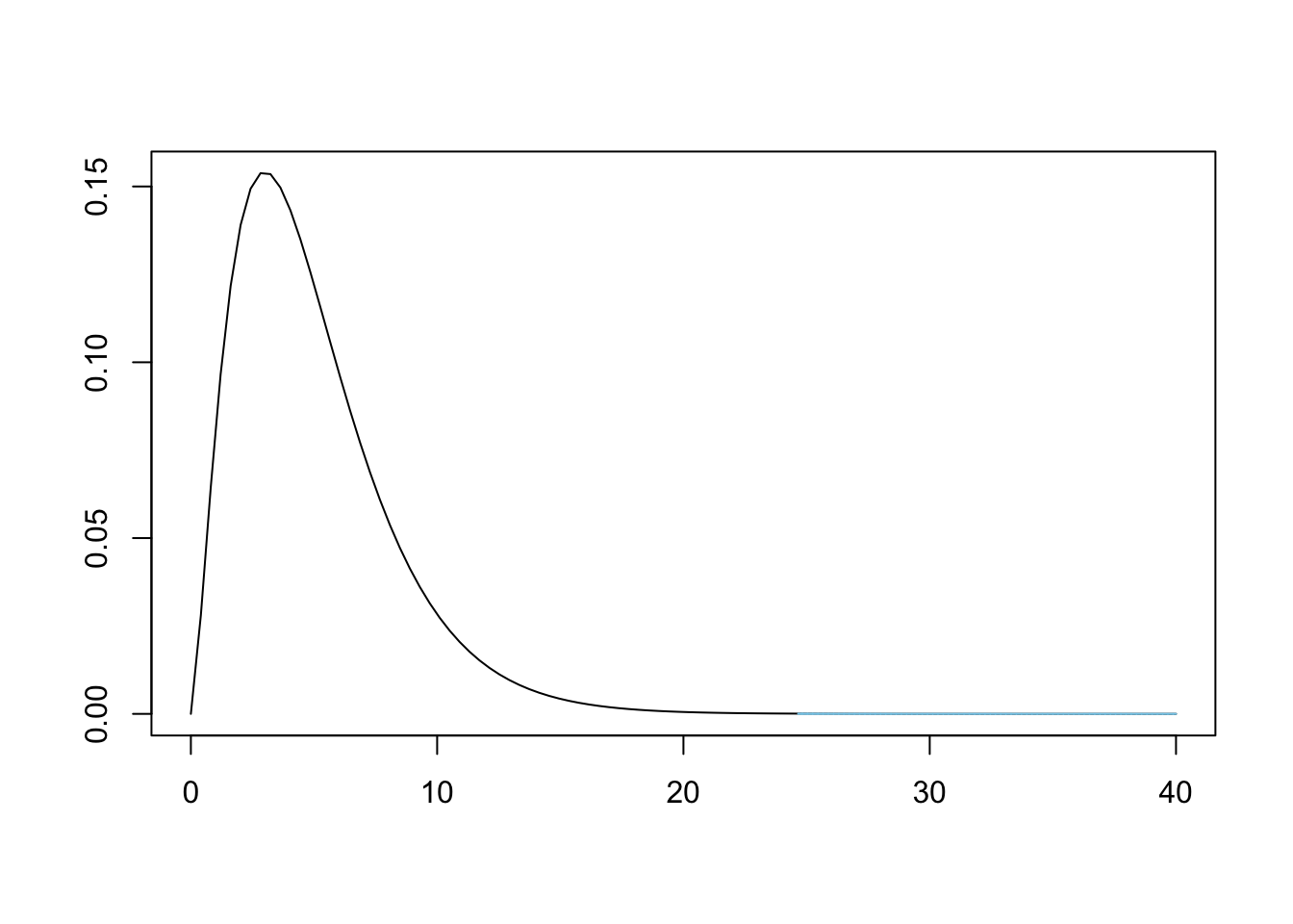
Figure 11.11: Chi Squared for Bag A and New Jersey

To find the area bound by this part of the \(\chi^2\) curve, that is calculate \(P( \chi^2 > X^2)\), we need a new function, pchisq(), which is the distribution function for the \(\chi^2\) distribution.

The syntax of pchisq() is

#This code will not run unless the necessary values are inputted.
pchisq( q, df, lower.tail )     

where the arguments are:

• q: The quantile that sets \(P(\chi^2 < q)\) or \(P( \chi^2 > q)\).

• df: The degrees of freedom being used for \(\chi^2\).

• lower.tail: This option controls whether the quantity returned is an upper or lower bound. If lower.tail = TRUE (or T), then the output is the quantity q such that \(P( \chi^2 \leq q ) = p\). If lower.tail is set to FALSE (or F), then the output is the quantity q such that \(P( \chi^2 > q ) = p\). If no value is set, R will default to lower.tail = TRUE.

Example 11.2 (M and Ms by Factory: Part 2) We can now find \(P( \chi^2 > X^2)\) for our value of \(X^2\) in Example 11.1, which is the \(p\)-value for our hypothesis test, with the following line of code.

pchisq( q = X2, df = degF, lower.tail = FALSE )

## [1] 0.6109161

We have a \(p\)-value that is greater than any reasonable level of significance, or \(\alpha\), This means that there is insufficient evidence to reject the assumption that \(p_k = \overline{p_k}\) for \({k = 1,2, \ldots, n}\) or that the population proportions that Bag A came from are that of the New Jersey factory. This, in an essence¹⁸⁷, says that it is more likely than not (\(p\)-value\(>0.5\)) that Bag A comes from the New Jersey factory.

The above work does not prove that Bag A came from the New Jersey factory, as it is impossible to prove a null hypothesis. However, this does say that we should not rule out New Jersey as the the factory that made Bag A.

To conduct a \(\chi^2\)-test of Proportions “by hand,” use the following Code Template. The only displayed value will be the \(p\)-value achieved, but all intermediate calculations will be saved to your environment.

#Save the frequencies as `data`
data <- 
#Save the assumed proportions as `prop`
prop <-
#The rest of the code just needs to be run
size <- sum( data )
Expected <- size * prop
Observed <- data
degF <- length( Observed )-1
Deviations <- Observed - Expected
Contributions <- (Deviations)^2/Expected
X2 <- sum( Contributions )
pchisq( q = X2, df = degF, lower.tail = FALSE )

We will first streamline our process by using the power of R before proceeding to try and rule out the possibility that Bag A came from the Tennessee factory.

11.3 chisq.test()

it is the aim of this book to show how calculations can be done “manually” using R to carry the weight of the calculations. However, in nearly every instance, there is an R function that can automate a lot of the work. Our newest function which will expedite our process is chisq.test().

The syntax of chisq.test() is

#This code will not run unless the necessary values are inputted.
chisq.test( x, p )     

where the arguments are:

• x: A numeric vector or matrix.

• p: A vector of probabilities of the same length as x.

If you are using chisq.test() to test if all probabilities are the equal, then you do not need to specify p.

In addition, there are many other arguments that can be used with chisq.test(), but we will not go into them here. See ?chisq.test if you are curious.

Example 11.3 (Is Bag A from New Jersey?) To quickly test Bag A came from the New Jersey factory, we simply run chisq.test as below

chisq.test( x = BagA, p = propNJ )

## 
##  Chi-squared test for given probabilities
## 
## data:  BagA
## X-squared = 3.5827, df = 5, p-value = 0.6109

or save the output of it to extract even more information from it as below.

test <- chisq.test( x = BagA, p = propNJ )

If test is the output of a chisq.test like above then you can get the following additional information:

• test$observed: The observed values or simply x.

• test$expected: The expected values found via the same method we did in the previous section.

• test$residuals^2: The contribution to \(\chi^2\) from each observed value.¹⁸⁸

With test still being the same rest run above, we get the following results which match our by hand calculations from Example 11.1.

test$observed

## [1]  59 119  75  60 126  69

test$expected

## [1]  63.5 127.0  63.5  63.5 127.0  63.5

#Note that we have rounded to 4 decimal places.
round( test$residuals^2, 4 )

## [1] 0.3189 0.5039 2.0827 0.1929 0.0079 0.4764

While using this method may be easier to find the \(X^2\) contributions, the main result we want from our software in a hypothesis test is a \(p\)-value. We can obtain this value by either running either test$p.value or simply running test. We will look at test as it also gives the \(X^2\) value as well as the degrees of freedom.

test

## 
##  Chi-squared test for given probabilities
## 
## data:  BagA
## X-squared = 3.5827, df = 5, p-value = 0.6109

What other information is saved within test as created in Example 11.3? That is, if you type test$ into an R script or your Console, what variables are you able to select from?

Example 11.4 (Is Bag A from Tennessee?) To see if we can really be confident that Bag A was made in New Jersey, we now test Bag A against the proportions used at the Tennessee factory.

test <- chisq.test( x = BagA, p = propTN )
test$observed

## [1]  59 119  75  60 126  69

We will look at the expected values and use the function round() to make the output easier to compare (and because we don’t want fractional \(\text{M}\&\text{M}\)s).

round( test$expected )

## [1]  67 104  69 101 105  63

We see some large deviations from the observed value, so we expect a large \(X^2\) and thus a small \(p\)-value. We can check this by simply looking at test.

test

## 
##  Chi-squared test for given probabilities
## 
## data:  BagA
## X-squared = 24.657, df = 5, p-value = 0.0001623

Recall that when we start a hypothesis test, we assume the conditions in \(H_0\). That is, we assumed that Bag A did come Tennessee. However, our analysis then gave us a \(p\)-value of 0.0001623. This is illustrated below.

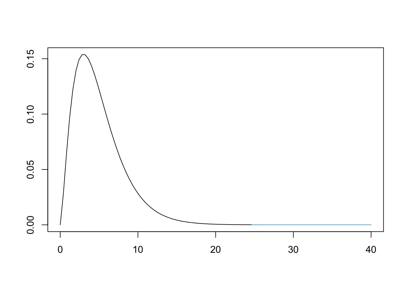
Figure 11.12: Chi Squared for Bag A and Tennessee

This means that we have sufficient evidence, at any reasonable level of significance, to conclude that Bag A does not come from a population whose proportions match that of the ones used at the Tennessee factory.

Since we are working under the assumption that there are only two factories making these candies, we can now be reasonably confident that Bag A did come from New Jersey as we ruled out the possibility of Bag A being made in Tennessee and have insufficient evidence to rule out the New Jersey factory.

We are only saying that we are confident that Bag A came from New Jersey explicitly because we are working under the assumption that there are only two factories that could have made Bag A.

Example 11.5 (Where is Bag B From?) We can first test Bag B against the New Jersey factory. We will do this quickly, but will include the observed and expected values so that we can compare cases with large and small \(p\)-values.

test <- chisq.test( x = BagB, p = propNJ )
test$observed

## [1]  62  95  76 114 107  70

test$expected

## [1]  65.5 131.0  65.5  65.5 131.0  65.5

test

## 
##  Chi-squared test for given probabilities
## 
## data:  BagB
## X-squared = 52.382, df = 5, p-value = 4.505e-10

This gives us sufficient evidence to abandon the assumption that Bag A was made at the New Jersey factory. This means that we are sufficiently convinced that Bag A came from the Tennessee factory. To confirm our belief that Bag B is from Tennessee, we will test BagB against propTN.

test <- chisq.test( x = BagB, p = propTN )
test$observed

## [1]  62  95  76 114 107  70

test$expected

## [1]  68.644 107.420  70.740 103.752 108.468  64.976

test

## 
##  Chi-squared test for given probabilities
## 
## data:  BagB
## X-squared = 3.8908, df = 5, p-value = 0.5652

Like before, we can loosely interpret this to mean that it is more likely than not (\(p\)-value\(>0.5\)) that Bag B comes from the Tennessee factory.

Again, working under the assumption that there are only two factories making these candies, this means we can be fairly confident that Bag B was made at the Tennessee factory.

11.4 Chi Squared Test of Independence

The \(\chi^2\) distribution can also be used to test if two categorical types of data are independent. That is, for example, does the distribution of eye color depend on a person’s gender. If these variables were independent, then the population proportion of eye color would not change if we looked at a specific gender or the entire population.

The hypothesis test we will run is as follows.

Theorem 11.2 The \(\chi^2\) distribution can be used to make the following hypothesis test.

\[\begin{align*} H_0 :&\; \text{The population proportions for different categories}\\ {} &\;\; \text{are the same for all of the populations.}\\ H_a :&\; \text{The population proportions for different categories}\\ {} &\;\; \text{are NOT the same for all of the populations.} \end{align*}\]

That is, we are seeing if the population proportion for different categories is independent of the different populations. If we view this in the mindset of \(\text{M}\&\text{M}\) colors, we are testing to see if different bags have the same color (category) proportions, i.e. that they come from the same factory. We will again calculate a \(\chi^2\)-statistic, still denoted \(X^2\) or X2, and get a \(p\)-value from it.

Essentially, we are now looking at a table of values and are trying to see if the proportions differ on different rows. In order to use Definition 11.3, we need to find \(P(\text{cell})\) and \(n\). The latter is easy as we can use the total number of observations in our table as \(n\). We will call this value \(\text{Table Total}\) to make our calculations clear.

When running a \(\chi^2\)-test of Independence:

• the assumption, \(H_0\), is that the two variables are independent
• the claim, \(H_a\), is that the two variables are dependent on one another

If the \(p\)-value falls at or below the level of significance, \(\alpha\), then we can reject our assumption and state that we have sufficient evidence (at this level of significance) to conclude that the claim, \(H_a\) is true.

If the \(p\)-value is greater than \(\alpha\), then we have insufficient evidence to abandon the assumption contained in \(H_0\).

Example 11.6 We begin by loading a data frame called Titanic.Dataset.

Use the following code to download TitanicDataset.

Titanic.Dataset <- read.csv( "https://statypus.org/files/Titanic.Dataset.csv" ) 

We can get more information about this dataset by looking at a dictionary for it at https://www.kaggle.com/c/titanic/data. This explains the meaning of the variables and tells us that the Sex variable indicates the gender of the passenger and the Pclass variable refers to the passenger class of the individual.

A question we can ask is if males and females were divided among the three passenger classes independently. That is, did males and females separate into the three passenger classes in different proportions. Below is the two way table for the Sex and Pclass variables.

table( Titanic.Dataset$Sex, Titanic.Dataset$Pclass )

##         
##            1   2   3
##   female  94  76 144
##   male   122 108 347

It is clear that we cannot expect that our sample to give exact equivalence of the category proportions for males and females, but we can assume that the variables are independent and see if our data is sufficient to show that that assumption is unfounded. That is, we have the following hypothesis test.

\[\begin{align*} H_0 :&\; \text{The population proportions for different passenger}\\ {} &\;\; \text{classes are the same for each gender.}\\ H_a :&\; \text{The population proportions for different passenger}\\ {} &\;\; \text{classes are NOT the same for each gender.} \end{align*}\]

We will continue this investigation in Example 11.10

As we are assuming that the rows of our table are independent, we can use the rule that \(P(\text{cell}) = P(\text{row})\cdot P(\text{column})\)¹⁸⁹ to find the probability of an arbitrary cell. Again, using our assumption, we can use the row and column relative frequencies to find estimate each of those probabilities. This gives us the following.

\[\begin{align*} P(\text{cell}) &= P(\text{row})\cdot P(\text{column})\\ {} &= \frac{\text{Row Total}}{\text{Total}} \cdot \frac{\text{Column Total}}{\text{Total}}\\ {} &= \frac{(\text{Row Total})\cdot (\text{Column Total}) }{(\text{Table Total})^2} \end{align*}\]

This then gives the following for \(\text{Exp}\).

\[\begin{align*} \text{Exp} &= P(\text{cell})\cdot (\text{Table Total})\\ {} &= \frac{(\text{Row Total})\cdot (\text{Column Total}) }{(\text{Table Total})^2} \cdot \text{Table Total}\\ {} &= \frac{(\text{Row Total})\cdot (\text{Column Total}) }{\text{Table Total}} \end{align*}\]

That is, to calculate the expected value of each cell, we need to calculate the row total times the column total and then divided by the table total for each cell. We summarize this work in the following definition.

Definition 11.5 Given a table of data, we can calculate the Expected Value of the Cell to be \(P(\text{cell})\) multiplied by \(\text{Table Total}\). Since we assume that the rows and columns are independent, we have that \[P(\text{cell}) = \frac{(\text{Row Total})\cdot (\text{Column Total}) }{(\text{Table Total})^2}\] and \[\text{Exp} = \frac{(\text{Row Total})\cdot (\text{Column Total}) }{\text{Table Total}}.\]

11.4.1 Calculating \(X^2\) By Hand

In this section, we will be looking at 4 different bags of \(\text{M}\&\text{M}\)s. The first 3 bags were bought at a local convenience store while the fourth bag, called the mystery bag, was mailed to you by your sweet Grandma because she knows how much you love \(\text{M}\&\text{M}\)s.

Use the following code to download MandMTable.

MandMTable <- read.csv( "https://statypus.org/files/MandMTable.csv" )

We begin by looking at the dataset containing all the information about all four bags.

MandMTable

##             X Red Orange Yellow Green Blue Brown
## 1       Bag 1  63    130     68    67  115    63
## 2       Bag 2  79    126     77    63  120    62
## 3       Bag 3 166    303    154   134  290   154
## 4 Mystery Bag  78    113     66    95  100    64

The hypothesis test we introduced above will assume that the bags come from populations where the proportions are equal for each color, i.e. that they call came from the same factory.

\[\begin{align*} H_0 :&\; \text{The population proportions for different colors}\\ {} &\;\; \text{are the same for all of the bags.}\\ H_a :&\; \text{The population proportions for different colors}\\ {} &\;\; \text{are NOT the same for all of the bags.} \end{align*}\]

Our \(p\)-value will then give us a measure of the likelihood that the deviations we encounter can be attributed solely to chance.

We will first test if the 3 bags we bought at the convenience store come from the same factory. The first two bags were pound size bags while the third bag was a party size bag which is nearly 2.5 pounds. To do our analysis, we first need to cut the data down to just the values we want to test. We can do this by choosing all three rows (1:3) and only columns 2 through 7 (2:7) which omits the column where we named the bags.

data <- MandMTable[ 1:3, 2:7 ]
data

##   Red Orange Yellow Green Blue Brown
## 1  63    130     68    67  115    63
## 2  79    126     77    63  120    62
## 3 166    303    154   134  290   154

To do the analysis by hand, we need the data to be in the matrix format. To see if this is the case, we can use the structure function, str().

str( data )

## 'data.frame':    3 obs. of  6 variables:
##  $ Red   : int  63 79 166
##  $ Orange: int  130 126 303
##  $ Yellow: int  68 77 154
##  $ Green : int  67 63 134
##  $ Blue  : int  115 120 290
##  $ Brown : int  63 62 154

We see that data is in the data.frame format and this will cause issues with the functions we need for our manual analysis. We can rectify this with the as.matrix() function.

The as.matrix() function attempts to turn its argument into a matrix.

data <- as.matrix( data )
data

##   Red Orange Yellow Green Blue Brown
## 1  63    130     68    67  115    63
## 2  79    126     77    63  120    62
## 3 166    303    154   134  290   154

This shows that the information stored in data has not changed. To see if as.matrix was successful, we can again use str.

str(data)

##  int [1:3, 1:6] 63 79 166 130 126 303 68 77 154 67 ...
##  - attr(*, "dimnames")=List of 2
##   ..$ : chr [1:3] "1" "2" "3"
##   ..$ : chr [1:6] "Red" "Orange" "Yellow" "Green" ...

While RStudio doesn’t explicitly state that data is in the matrix format, the string int [1:3, 1:6] means that data is a matrix with integer values with rows numbered 1 to 3 and columns numbered from 1 to 6.

To begin our analysis, we need to append row and column totals. In its most simple usages, this is exactly what the addmargins() function does. We will save the output as dataW to remind us it is our data With totals appended.

The addmargins() function will append row and column totals to a matrix.

dataW <- addmargins( data )
dataW

##     Red Orange Yellow Green Blue Brown  Sum
## 1    63    130     68    67  115    63  506
## 2    79    126     77    63  120    62  527
## 3   166    303    154   134  290   154 1201
## Sum 308    559    299   264  525   279 2234

We see from this that the first bag had 506 \(\text{M}\&\text{M}\)s, the second bag had 527 \(\text{M}\&\text{M}\)s, and the third bag, the Party Size, had 1201 \(\text{M}\&\text{M}\)s. We also see that we had a total of 2234 \(\text{M}\&\text{M}\)s in the three convenience store bags. The least common color was Green with a total of 264 and the most common color was orange with a total of 559.

As we saw in Definition 11.5, to calculate the expected value of each cell, we need to calculate the row total times the column total and then divided by the table total for each cell. We can do this by pulling out the row and column totals using the marginSums() function.

The syntax of marginSums() is

#This code will not run unless the necessary values are inputted.
marginSums( x, margin )     

where the arguments are:

• x: An array.

• margin: For our use: 1 indicates rows, 2 indicates columns.

We can find the row and column totals now.

rows <- marginSums( data, 1 )     
#marginSums output as column vector
rows

##    1    2    3 
##  506  527 1201

We invoke the function t() which turns the output of marginSums (which is a column vector) into a row vector for the column totals.

The t() function finds the transpose of a matrix. One simple example is that t will change a column vector into a row vector (or vice versa).

columns <- t( marginSums( data, 2 ) ) 
#t() transposes column to row vector
columns

##      Red Orange Yellow Green Blue Brown
## [1,] 308    559    299   264  525   279

R shows us that columns is a row vector by labeling it with [1,] in front of the values. This indicates that the entries are the values of the 1st row of a table.

To create a matrix which is composed of values of the product of the row total and the column total for each cell, we need to invoke, yet another, new tool. This time it is the operation which computes matrix multiplication %*%.

The operation M %*% N does the matrix multiplication of M and N.

Example 11.7 As a quick example of the %*% operator, we can define the following vector OneToNine to be as follows.

OneToNine <- 1:9
OneToNine

## [1] 1 2 3 4 5 6 7 8 9

If we then look at the operation OneToNine %*% t(OneToNine) (where we use t() to convert the second copy of OneToFive to a row vector), we get the classic multiplication chart.

OneToNine %*% t( OneToNine )

##       [,1] [,2] [,3] [,4] [,5] [,6] [,7] [,8] [,9]
##  [1,]    1    2    3    4    5    6    7    8    9
##  [2,]    2    4    6    8   10   12   14   16   18
##  [3,]    3    6    9   12   15   18   21   24   27
##  [4,]    4    8   12   16   20   24   28   32   36
##  [5,]    5   10   15   20   25   30   35   40   45
##  [6,]    6   12   18   24   30   36   42   48   54
##  [7,]    7   14   21   28   35   42   49   56   63
##  [8,]    8   16   24   32   40   48   56   64   72
##  [9,]    9   18   27   36   45   54   63   72   81

We can now use the %*% operation to help us find the expected values of each of the cells of our array for the \(\text{M}\&\text{M}\)s. We do this by using the %*% operation with the vectors rows and columns which we have already defined.¹⁹⁰ The result is a matrix with the same dimensions of data which contains the row total multiplied by the column total in each cell.

rows %*% columns

##      Red Orange Yellow  Green   Blue  Brown
## 1 155848 282854 151294 133584 265650 141174
## 2 162316 294593 157573 139128 276675 147033
## 3 369908 671359 359099 317064 630525 335079

To obtain the expected values, we simply divide the result by the total count of the data which we can do by using sum( data ). We round the result to make the table easier to read.

Expected <- ( rows %*% columns ) / sum( data )  
round( Expected )                           

##   Red Orange Yellow Green Blue Brown
## 1  70    127     68    60  119    63
## 2  73    132     71    62  124    66
## 3 166    301    161   142  282   150

Similar to the previous section, we can now calculate the deviation of each cell by subtracting the expected value from the observed count we have in the matrix data.

Deviations <- data - Expected
Deviations

##          Red   Orange     Yellow      Green      Blue      Brown
## 1 -6.7618621  3.38675  0.2766338  7.2041182 -3.912265 -0.1933751
## 2  6.3428827 -5.86795  6.4659803  0.7224709 -3.847359 -3.8160251
## 3  0.4189794  2.48120 -6.7426141 -7.9265891  7.759624  4.0094002

Up until this point, we haven’t discussed the degrees of freedom we will use. The degrees of freedom that we use is the smallest number of deviations needed to create all of the deviations. If we append row and column totals, we see that we have 0 totals in every row and column.

#Rounded to 8 decimal places
DeviationsW <- round( addmargins(Deviations), 8 ) 
DeviationsW                                       

##            Red   Orange     Yellow      Green      Blue      Brown Sum
## 1   -6.7618621  3.38675  0.2766338  7.2041182 -3.912265 -0.1933751   0
## 2    6.3428827 -5.86795  6.4659803  0.7224709 -3.847359 -3.8160251   0
## 3    0.4189794  2.48120 -6.7426141 -7.9265891  7.759624  4.0094002   0
## Sum  0.0000000  0.00000  0.0000000  0.0000000  0.000000  0.0000000   0

It turns out that we can remove an entire row and column of deviations and recreate the rest. If we look at the first 2 rows and the first 5 columns and append row/column totals, we see that the last row and column values can be found via this method.¹⁹¹

addmargins( Deviations[ 1:2, 1:5 ] )

##            Red   Orange    Yellow     Green      Blue       Sum
## 1   -6.7618621  3.38675 0.2766338 7.2041182 -3.912265 0.1933751
## 2    6.3428827 -5.86795 6.4659803 0.7224709 -3.847359 3.8160251
## Sum -0.4189794 -2.48120 6.7426141 7.9265891 -7.759624 4.0094002

This shows that we need only one less row and one less column to predict all the deviations and we end up validating the formula that the degrees of freedom is equal to \((R-1)(C-1)\) where \(R\) is the number of rows in our data and \(C\) is the number of columns.

We can easily obtain these values in general so that our code will work for any matrix saved into the variable data.

R <- nrow( data )
C <- ncol( data )
degF <- ( R - 1 ) * ( C - 1 )

The rest of the method is identical to that used for using \(X^2\) for proportions earlier. We first calculate the \(X^2\) contributions by dividing the square of the deviations by the expected value.

Contributions <- Deviations^2/Expected
Contributions

##           Red     Orange      Yellow       Green      Blue        Brown
## 1 0.655412256 0.09059144 0.001129983 0.867941354 0.1287152 0.0005917382
## 2 0.553726362 0.26111603 0.592748031 0.008381261 0.1195195 0.2212538253
## 3 0.001060168 0.02048575 0.282830074 0.442699390 0.2133350 0.1071753151

Our final \(\chi^2\)-statistic is then simply the sum of these values.

X2 <- sum( Contributions )
X2

## [1] 4.568713

Using the degrees of freedom and \(X^2\) (X2 when in R) above, we can now look at how rare X2 is on the \(\chi^2\) distribution.

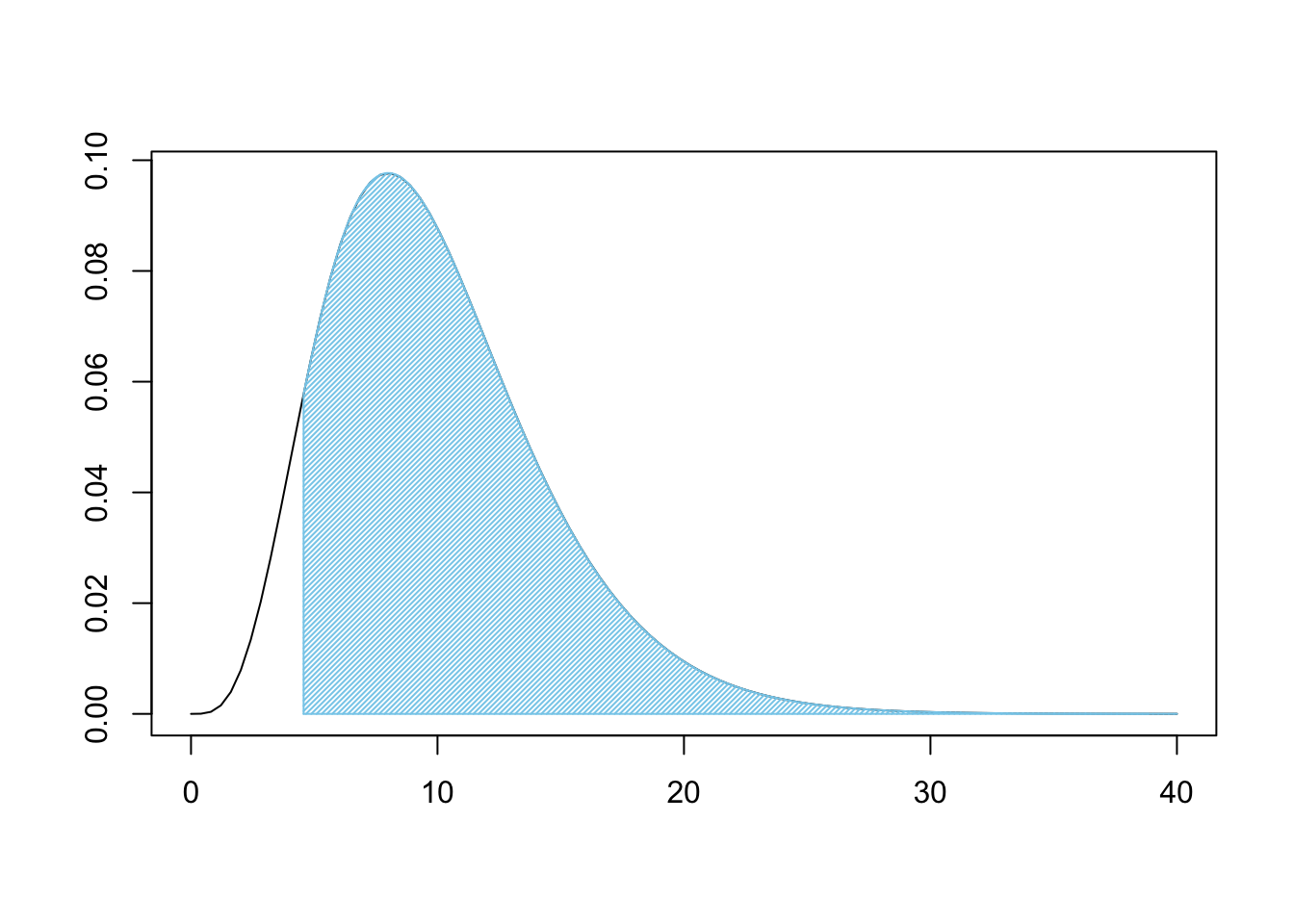
Figure 11.13: Chi Squared for Three Bags

This is a very large shaded area. Like before, we can use pchisq to find the shaded area.

pchisq( q = X2, df = degF, lower.tail = FALSE )

## [1] 0.9180675

If we were 100% certain of \(H_0\) prior to our analysis, we are still over 91.8% belief in \(H_0\). That is, under the assumption of independence, we would get samples that are at least as different from expected values as ours was over 91.8% of the time. This means that we do not have good reason to believe that the bags come from different populations. That is, the claim that they were all produced at different factories has very little support.

We don’t know which factory the bags were made at by any of this, nor did we assume any factory distribution at any point or our analysis. We are simply comparing the bags to each other and do not need to define any probabilities.

We can summarize the above techniques in the following Code Template.

To conduct a \(\chi^2\)-test of Independence “by hand,” use the following Code Template. The only displayed value will be the \(p\)-value achieved, but all intermediate calculations will be saved to your environment.

#Save the table as `data`
data <- 
#The rest of the code just needs to be run
data <- as.matrix( data )
Expected <- size * prop
rows <- marginSums( data, 1 )
#t() transposes column to row vector
columns <- t( marginSums( data, 2 ) ) 
Expected <- ( rows %*% columns ) / sum( data )
Observed <- data
R <- nrow( data )
C <- ncol( data )
degF <- ( R - 1 ) * ( C - 1 )
Deviations <- Observed - Expected
Contributions <- (Deviations)^2/Expected
X2 <- sum( Contributions )
pchisq( q = X2, df = degF, lower.tail = FALSE )

11.4.2 With chisq.test

As before, chisq.test can automate nearly all of our work thus far. We will show how to apply it with the following example.

Example 11.8 (Testing the First 3 Bags) We can test the three bags bought at the convenience store using chisq.test. It is worthy of note that we do not need to make certain that our data is in the matrix format if we don’t care to do the step-by-step calculations as before. As such, we can simply set data to be the applicable portion of MandMTable.

data <- MandMTable[ 1:3, 2:7 ]
data

##   Red Orange Yellow Green Blue Brown
## 1  63    130     68    67  115    63
## 2  79    126     77    63  120    62
## 3 166    303    154   134  290   154

As we have already made all the calculations by hand, we can simply run the single line of code below to confirm it yields the same analysis we achieved “by hand.”

chisq.test( data )

## 
##  Pearson's Chi-squared test
## 
## data:  data
## X-squared = 4.5687, df = 10, p-value = 0.9181

As before, this absurdly high \(p\)-value means that we are unable to prove anything as we are left with more belief in \(H_0\) which we assumed was true and thus cannot be proven to be true.

When using chisq.test() for a test of independence, we do not need to provide a value for p as we are simply testing if the data come from some common, yet unknown, collection of proportions.

Example 11.9 (What about the Mystery Bag?) Now that we have a much quicker path to hypothesis test results, we can investigate the Mystery Bag that your Grandma sent. That is, we want to test if all four bags come from the same population, i.e. that they were made at the same factory. Remember that we assume that the bags do come from the same population (factory) in all of our analysis. To begin the test, we set data to be all of the numeric portion of MandMTable. That is, we set data to be the first 4 rows and the last 6 columns.

data <- MandMTable[ 1:4, 2:7 ]
data

##   Red Orange Yellow Green Blue Brown
## 1  63    130     68    67  115    63
## 2  79    126     77    63  120    62
## 3 166    303    154   134  290   154
## 4  78    113     66    95  100    64

We could simply run the single line chisq.test( data ), but as we have not made any of the calculations, we will save this as test so we can extract more information from it if we want to.

test <- chisq.test( data )
test

## 
##  Pearson's Chi-squared test
## 
## data:  data
## X-squared = 23.86, df = 15, p-value = 0.0675

Looking at test we see that we have 15 degrees of freedom as expected and a \(p\)-value of 0.0675. While this is not below the classic value of \(\alpha = 0.05\), it is significantly closer than the \(p\)-value obtained from just the bags bought at the convenience store. The inclusion of the Mystery Bag drastically reduced the value of \(p\)-value. We should only expect to see at least this much deviation from expected values in 6.75% of samples, or we can roughly state that we only have a 6.75% belief in \(H_0\) after our analysis. But why did that happen? We can look at the expected values under the assumption that all four bags came from the same factory and the resulting \(X^2\) contributions.

round( test$expected )

##   Red Orange Yellow Green Blue Brown
## 1  71    124     67    66  115    63
## 2  74    129     70    69  120    66
## 3 169    293    159   157  273   150
## 4  72    126     68    67  117    64

round( test$residuals^2, 2 )       # Rounds the contributions to 2 decimal places

##    Red Orange Yellow Green Blue Brown
## 1 0.91   0.33   0.01  0.01 0.00  0.00
## 2 0.34   0.06   0.71  0.49 0.00  0.21
## 3 0.04   0.31   0.18  3.31 1.06  0.12
## 4 0.43   1.36   0.09 11.34 2.54  0.00

We see that the Green \(\text{M}\&\text{M}\)s seem to be the big issue here. A \(X^2\) contribution of over 11 in one cell is definitely a major contributor to \(\chi^2\)-statistic, in fact that one cell accounts for nearly half of the statistic which was 23.86. We can plot \(X^2\) to see how rare it looks.

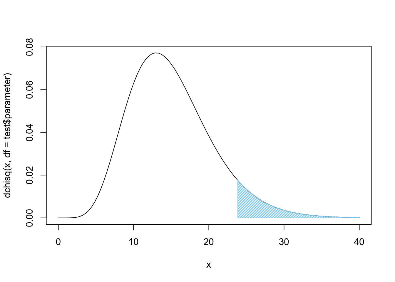
Figure 11.14: Chi Squared for all Four Bags

Again, this, unfortunately, does not offer sufficient evidence at the \(\alpha = 0.05\) level of significance, but it does offer fairly strong evidence that these four bags do not come from the same population, i.e. they do not come from the same factory.

Example 11.10 (Gender vs. Class on the Titanic) Here we continue the investigation we started in Example 11.6 to test if the variables of Sex and Pclass are independent. To compactify our code and make it a bit easier to read, we will create a copy of Titanic.Dataset which we call dd to make our calculations.

dd <- Titanic.Dataset

This is an example of a working copy like we introduced in Example 1.25 way back in Chapter 1. To get a handle on the types of information in our dataset, we use the str function.

str( dd )

## 'data.frame':    891 obs. of  12 variables:
##  $ PassengerId: int  1 2 3 4 5 6 7 8 9 10 ...
##  $ Survived   : int  0 1 1 1 0 0 0 0 1 1 ...
##  $ Pclass     : int  3 1 3 1 3 3 1 3 3 2 ...
##  $ Name       : chr  "Braund, Mr. Owen Harris" "Cumings, Mrs. John Bradley (Florence Briggs Thayer)" "Heikkinen, Miss. Laina" "Futrelle, Mrs. Jacques Heath (Lily May Peel)" ...
##  $ Sex        : chr  "male" "female" "female" "female" ...
##  $ Age        : num  22 38 26 35 35 NA 54 2 27 14 ...
##  $ SibSp      : int  1 1 0 1 0 0 0 3 0 1 ...
##  $ Parch      : int  0 0 0 0 0 0 0 1 2 0 ...
##  $ Ticket     : chr  "A/5 21171" "PC 17599" "STON/O2. 3101282" "113803" ...
##  $ Fare       : num  7.25 71.28 7.92 53.1 8.05 ...
##  $ Cabin      : chr  "" "C85" "" "C123" ...
##  $ Embarked   : chr  "S" "C" "S" "S" ...

We continue by recreating the two-way table of our variables and save it as data below.

data <- table( dd$Sex, dd$Pclass )
data

##         
##            1   2   3
##   female  94  76 144
##   male   122 108 347

Before looking at the end result of our hypothesis test, we can save the output into test and look at some of its components.

test <- chisq.test( data )

Recall that we assumed that the proportion in each class would be the same for both males and females. Under this assumption, below is the counts we should have expected, rounded to the nearest person.

round( test$expected )

##         
##            1   2   3
##   female  76  65 173
##   male   140 119 318

It is not easy to determine just how much our observed values, data, differ from the above. However, we can look at the square of the residuals portion of test to see the \(X^2\) contribution of each cell (rounded to 3 decimal places).

round( test$residuals^2, 3 )                    #Gives (O - E)^2/E

##         
##              1     2     3
##   female 4.199 1.919 4.872
##   male   2.285 1.044 2.651

While these values are not as high as the contribution of over 11 in the \(\text{M}\&\text{M}\) example, it is mindful to recall that we are only working with \((2-1)(3-1) = 1\cdot 2= 2\) degrees of freedom. We can then simply call test to see the result of the hypothesis test.

test

## 
##  Pearson's Chi-squared test
## 
## data:  data
## X-squared = 16.971, df = 2, p-value = 0.0002064

This test assumed that the variables Pclass and Sex were independent. Under this assumption, we would only expect to get a sample that deviates from the expected values as much as ours does only 0.02% of the time! This is sufficient evidence that we can no longer maintain our belief in \(H_0\) and can reject it and accept \(H_a\) that states that an individual’s passenger class and gender are related. That is, the proportion of each class differs for males and females.

Example 11.11 (When Data Needs Cleaned Up) It is important to note that data often needs “cleaned up.” If we wanted to see if there was a different proportion of males and females at each of the ports that the Titanic sailed from before leaving Europe (refer to the dictionary link above for more information), we would begin by creating a two-way table of the variables Sex and Embarked.

data <- table( dd$Sex, dd$Embarked )
#Contains blank cells in first column
data                                  

##         
##                C   Q   S
##   female   2  73  36 203
##   male     0  95  41 441

We see that there are 2 females who do not have a port of embarkation listed. If we tried to do our analysis on the entire table, we would encounter issues.¹⁹² To rectify this, we could attempt to correct the dataset and this process is explained and done in the Appendix, Section 11.5.3. Alternatively, we could simply remove the unknown port portion of our data as below.

#Removes first column of blank values for embarked
data <- data[ , 2:4 ]             
#Cleaned up table
data                                  

##         
##            C   Q   S
##   female  73  36 203
##   male    95  41 441

Now that we have a table of only the values we wish to test, we can invoke chisq.test to see if an equal proportion of males and females boarded at each of the three ports that the Titanic used.

chisq.test( data )

## 
##  Pearson's Chi-squared test
## 
## data:  data
## X-squared = 13.356, df = 2, p-value = 0.001259

If a person’s gender was independent of the port they embarked from, we would only expect to get data such as ours about 0.13% of the time. This is sufficient evidence that our assumption, \(H_0\), can be rejected and we can conclude that males and females boarded the titanic at different proportions at least one of the ports. That is, we have sufficient evidence that the variables Sex and Embarked are dependent variables.

Review for Chapter 11

Definitions

Section 11.1

Definition 11.1 \(\;\) Given a vector \({\bf x} = ( x_1, x_2, \ldots, x_n )\) having \(n\) values (with \(n\geq 2\)), we define the Scaled Sample Variance, denoted \(\text{SSV}\), to be the product of the Sample Variance and the Degrees of Freedom (See Definition 4.8).

\[\text{SSV} = (n-1)\cdot s ^2 = \sum (x - \bar{x})^2\]

Definition 11.2 \(\;\) For any positive integer \(\nu\), the \(\chi^2\) Distribution with \(\nu\) Degrees of Freedom is the distribution of the scaled sample variances of samples of size \(n = \nu + 1\) from \(\text{Norm}(0,1)\).

Definition 11.3 \(\;\) Given a table of values pulled from a sample, we call the cells of the table the Observed Value of the Cell and will denote them as \(\text{Obs}\) in our calculations. We define the \({\bf \chi^2 }\)-statistic, denoted by \(X^2\), to be given by

\[ X^2 = \sum_{\text{all cells}} \frac{\left(\text{Obs} - \text{Exp}\right)^2}{\text{Exp}} \] where we define the Expected Value of the Cell, denoted as \(\text{Exp}\), to be

\[ \text{Exp} = P(\text{cell})\cdot n \] where \(P(\text{cell})\) is the probability of a random value satisfying the conditions of that cell under the assumed conditions.

Each summand of \(X^2\), i.e. a term of form \(\frac{\left(\text{Obs} - \text{Exp}\right)^2}{\text{Exp}}\), is called an \(\bf X^2\)-Contribution.

Section 11.2

Definition 11.4 \(\;\) Given a sample of \(n\) individuals broken into \(N\) different disjoint categories such that the count of the first category is \(x_1\), the count of the second category is \(x_2\), and so on. This implies that \(x_1 + x_2 + \cdots x_N = n\) and we can further define \(\widehat{p_k} = \frac{x_k}{n}\) so that \(\widehat{p_1} + \widehat{p_2} + \cdots \widehat{p_N} = 1.\)

The following gives an overview of the different proportions we have under consideration.

\[\begin{align*} p_k &= \text{True Population Proportion for category $k$ (True Parameter)}\\ \widehat{p_k} &= \frac{x_k}{n} = \text{Observed Sample Proportion for category $k$ (Statistic)}\\ \overline{p_k} &= \text{Assumed Population Proportion for category $k$ for $H_0$ (Assumed Parameter)} \end{align*}\]

Each of the \(N\) categories gives us a Cell and we say the values of \(x_k\) are the Observed Values, which we denoted \(\text{Obs}\) earlier. We can then define \(P(\text{Cell}) = \overline{p_k}\) for each \(k = 1, 2, \ldots N\). This gives that the Expected Values, which we denoted \(\text{Exp}\) earlier, are the values of \(\overline{p_k}\cdot n\) for all the values of \(k\).

Results

Section 11.2

Theorem 11.1 \(\;\) Given the hypothesis test with the setup of Definition 11.4 as shown below, \[\begin{align*} H_0 :&\; p_1 = \overline{p_1}\\ &\; p_2 = \overline{p_2}\\ &\; \vdots\\ &\; p_n = \overline{p_n}\\ H_a :&\; \text{At least one of the above statements is false,} \end{align*}\] the associated \(p\)-value is the area under the \(\chi^2\) distribution with \(n-1\) degrees of freedom for the values greater than the \(X^2\) statistic as defined in Definition 11.3.

Section 11.4

Theorem 11.2 \(\;\) The \(\chi^2\) distribution can be used to make the following hypothesis test.

\[\begin{align*} H_0 :&\; \text{The population proportions for different categories}\\ {} &\;\; \text{are the same for all of the populations.}\\ H_a :&\; \text{The population proportions for different categories}\\ {} &\;\; \text{are NOT the same for all of the populations.} \end{align*}\]

Big Ideas

Section 11.1

Like we have seen a few times now, parameters often use fancy Greek letters, such as \(\chi^2\), while their associated statistic often use similar Roman (your standard ABCs), such as \(X^2\). So far we have seen the following combinations:

\[\begin{align*} \textbf{S}\text{ample} &\approx \textbf{P}\text{opulation}\\ \textbf{S}\text{tatistic} &\approx \textbf{P}\text{arameter}\\ \textbf{S}\text{ort of } &\approx \textbf{P}\text{erfect}\\ \bar{x} &\approx \mu\\ s &\approx \sigma\\ \text{SE} &\approx \sigma_{\hat{p}}\\ X^2 &\approx \chi^2 \end{align*}\]

Section 11.2

In general, a hypothesis test is of form below. \[\begin{align*} H_0 &: \text{True Parameter} = \text{Assumed Parameter}\\ H_a &: \text{True Parameter} \; \Box \;\text{Assumed Parameter} \end{align*}\]

where \(\Box\) is chosen so that \(\text{Sample Statistic} \; \Box \; \text{Assumed Parameter}\) is true.

When running a \(\chi^2\)-test of Proportions:

• the assumption, \(H_0\), is that our data agrees with the assumed proportions
• the claim, \(H_a\), is that our data does not agree with the assumed proportions

If the \(p\)-value falls at or below the level of significance, \(\alpha\), then we can reject our assumption and state that we have sufficient evidence (at this level of significance) to conclude that the claim, \(H_a\) is true.

If the \(p\)-value is greater than \(\alpha\), then we have insufficient evidence to abandon the assumption contained in \(H_0\).

Section 11.4

When running a \(\chi^2\)-test of Independence:

• the assumption, \(H_0\), is that the two variables are independent
• the claim, \(H_a\), is that the two variables are dependent on one another

If the \(p\)-value falls at or below the level of significance, \(\alpha\), then we can reject our assumption and state that we have sufficient evidence (at this level of significance) to conclude that the claim, \(H_a\) is true.

If the \(p\)-value is greater than \(\alpha\), then we have insufficient evidence to abandon the assumption contained in \(H_0\).

Important Remarks

Section 11.2

In Theorem 11.1, it is required that \(p_1 + p_2 + \cdots + p_n = 1\). If not, we cannot use the methods here and would need to use prop.test(). See Section 9.6, in particular Example 9.34, for more information.

Section 11.3

If you are using chisq.test() to test if all probabilities are the equal, then you do not need to specify p.

Code Templates

Section 11.2

To conduct a \(\chi^2\)-test of Proportions “by hand,” use the following Code Template. The only displayed value will be the \(p\)-value achieved, but all intermediate calculations will be saved to your environment.

#Save the frequencies as `data`
data <- 
#Save the assumed proportions as `prop`
prop <-
#The rest of the code just needs to be run
size <- sum( data )
Expected <- size * prop
Observed <- data
degF <- length( Observed )-1
Deviations <- Observed - Expected
Contributions <- (Deviations)^2/Expected
X2 <- sum( Contributions )
pchisq( q = X2, df = degF, lower.tail = FALSE )

Section 11.4

To conduct a \(\chi^2\)-test of Independence “by hand,” use the following Code Template. The only displayed value will be the \(p\)-value achieved, but all intermediate calculations will be saved to your environment.

#Save the table as `data`
data <- 
#The rest of the code just needs to be run
data <- as.matrix( data )
Expected <- size * prop
rows <- marginSums( data, 1 )
#t() transposes column to row vector
columns <- t( marginSums( data, 2 ) ) 
Expected <- ( rows %*% columns ) / sum( data )
Observed <- data
R <- nrow( data )
C <- ncol( data )
degF <- ( R - 1 ) * ( C - 1 )
Deviations <- Observed - Expected
Contributions <- (Deviations)^2/Expected
X2 <- sum( Contributions )
pchisq( q = X2, df = degF, lower.tail = FALSE )

New Functions

Section 11.2

The syntax of pchisq() is

#This code will not run unless the necessary values are inputted.
pchisq( q, df, lower.tail )     

where the arguments are:

• q: The quantile that sets \(P(\chi^2 < q)\) or \(P( \chi^2 > q)\).

• df: The degrees of freedom being used for \(\chi^2\).

• lower.tail: This option controls whether the quantity returned is an upper or lower bound. If lower.tail = TRUE (or T), then the output is the quantity q such that \(P( \chi^2 \leq q ) = p\). If lower.tail is set to FALSE (or F), then the output is the quantity q such that \(P( \chi^2 > q ) = p\). If no value is set, R will default to lower.tail = TRUE.

Section 11.3

The syntax of chisq.test() is

#This code will not run unless the necessary values are inputted.
chisq.test( x, p )     

where the arguments are:

• x: A numeric vector or matrix.

• p: A vector of probabilities of the same length as x.

Section 11.4

The as.matrix() function attempts to turn its argument into a matrix.

The addmargins() function will append row and column totals to a matrix.

The syntax of marginSums() is

marginSums( x, margin )     
#This code will not run unless the necessary values are inputted.

where the arguments are:

• x: An array.

• margin: For our use: 1 indicates rows, 2 indicates columns.

The t() function finds the transpose of a matrix. One simple example is that t will change a column vector into a row vector (or vice versa).

The operation M %*% N does the matrix multiplication of M and N.

Exercises

Exercise 11.1 If you are given a bag of \(\text{M}\&\text{M}\)s with the following color distribution, find the deviations as well as the \(X^2\) contributions for each of the colors when compared to the New Jersey factory using the proportions given in Example 11.1.

##    Red Orange Yellow  Green   Blue  Brown 
##     82    129     61     62    123     61

Exercise 11.2 Using the bag in the above problem, use a \(\chi^2\) Test of Proportions to try and figure out at which factory it was made following the methods outlined in Section 11.2.

Exercise 11.3 Use a \(\chi^2\) Test of Independence to see if a passenger on the Titanic’s survival was independent of their passenger class.

Exercise 11.4 Use a \(\chi^2\) Test of Independence to see if a passenger on the Titanic’s survival was independent of their gender.

11.5 Appendix

11.5.1 Alternate CLT

We first introduced the Central Limit Theorem, Theorem 9.1, in Section 9.1.3. There we formulated the distribution of the sample means, but it is also possible to formulate the same result based off of the sample sums as shown below.

Theorem 11.3 (Central Limit Theorem (Alternate Version)) Given a distribution with a population mean of \(\mu_x\) and a population standard deviation of \(\sigma_X\), then the collection of samples of size \(n\) gives rise to a distribution of sums, \(\Sigma\), which have mean and standard deviation given below. \[\begin{align*} \mu_{\Sigma} & = n \cdot \mu_x\\ \sigma_{\Sigma} & = \sqrt{n} \cdot \sigma_X \end{align*}\]

• If the original distribution was Normal, then the distribution of sample means is also Normal.

• However, the distribution approaches \(\text{Norm}( \mu_{\Sigma}, \sigma_{\Sigma})\) as \(n\) gets large regardless of the shape of the original distribution.

A great video by 3 Blue 1 Brown begins with this version and can be found on YouTube.

To demonstrate this version, we recall that a fair die has \(\mu_x = 3.5\) and \(\sigma_X = \sqrt{3.5}\). If we use \(\text{Norm}(3.5, \sqrt{3.5})\) as a model, we get the following distributions of \(\bar{x}\) for \(n = 1, 2, \ldots, 10\).

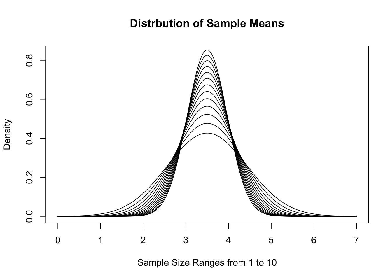
Figure 11.15: Distribution of Sample Means for Varied \(n\)

This visualization gives a good demonstration on why we call this the Central Limit Theorem. As \(n\) increases, the distribution gets tighter and tighter around the value \(\mu_x\). If we look at sample sums instead, we get the following distributions for the same sample sizes.

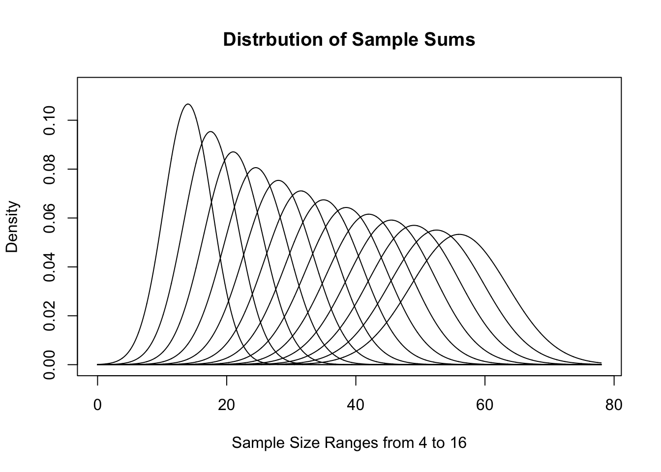
Figure 11.16: Distribution of Sample Sums for Varied \(n\)

These sets of graphs show different interpretations of effectively the same distribution. They have similarities to the distributions we saw for \(\chi^2\) earlier and show how different looking graphs can be essentially the same.

11.5.2 Why not prop.test

It is important to remember that we explicitly used the fact that the sum of the probabilities in Section 11.2. This is what allowed us to use \(n-1\) degrees of freedom to get a stronger result. If we were to try and use the function prop.test which we first encountered in Chapter 9, we would get the following for testing Bag A against the New Jersey factory.

prop.test( x = BagA, n = replicate(length(BagA), sum(BagA)), p = propNJ )

## 
##  6-sample test for given proportions without continuity correction
## 
## data:  BagA out of replicate(length(BagA), sum(BagA)), null probabilities propNJ
## X-squared = 4.192, df = 6, p-value = 0.6507
## alternative hypothesis: two.sided
## null values:
## prop 1 prop 2 prop 3 prop 4 prop 5 prop 6 
##  0.125  0.250  0.125  0.125  0.250  0.125 
## sample estimates:
##    prop 1    prop 2    prop 3    prop 4    prop 5    prop 6 
## 0.1161417 0.2342520 0.1476378 0.1181102 0.2480315 0.1358268

While the \(p\)-value found here is similar to that found in Section 11.2, it is not the same as we can quickly see that here, prop.test is using 6 degrees of freedom where chisq.test used df = 5. This happens because prop.test does not assume that the sum of the assumed proportions is 1.

Thus, when testing multiple proportions, if we know that we are looking at all possible cases of a population so that the sum of the assumed proportions is 1, we can invoke chisq.test and should leave prop.test for the types of questions we saw in Section 9.6.

11.5.3 Updating a Dataset

In Example 11.11 (where you can download the dataset if necessary), we saw that the Titanic.Dataset had missing values in the Embarked column. In this section, we show how to manually fix Titanic.Dataset$Embarked using a text editor as well as a spreadsheet program to update a dataset when new information can be found.

We begin by looking at the Embarked data using table.

table( Titanic.Dataset$Embarked )

## 
##       C   Q   S 
##   2 168  77 644

We can find who the basic information for the two passengers without values listed for Embarked with the following line of code where we also limit the output to only the first four columns so that it will display better here on the website.

Titanic.Dataset[ Titanic.Dataset$Embarked == "",  1:4 ]

##     PassengerId Survived Pclass                                      Name
## 62           62        1      1                       Icard, Miss. Amelie
## 830         830        1      1 Stone, Mrs. George Nelson (Martha Evelyn)

Doing an internet search for Titanic Icard, Miss. Amelie leads to many links including https://www.encyclopedia-titanica.org/titanic-survivor/amelia-icard.html. Reading the information on the page tells us that Amelie was the personal maid of the other passenger listed above, Mrs. Martha Stone.¹⁹³ It also tells us that both Amelia and Martha embarked on the Titanic from Southampton on Wednesday, 10 April, 1912. Thus, the values of Titanic.Dataset$Embarked should be "S" for both Amelie and Martha.

The first step of updating the dataset with either a text editor or spreadsheet program is to get the .csv file onto your computer. Simply pasting the following into a web browser should automatically download the file Titanic.Dataset.csv to your computer.

https://statypus.org/files/Titanic.Dataset.csv

You may also be able to simply click on this Link.

• Using a text editor: The first step is simply to open the file in an appropriate program as shown below.

It is best to use a simple text editor as compared to a fancier word processing program. Programs such as NotePad on Windows machines and TextEdit on Apple machines are recommended. Programs such as Microsoft Word are likely to modify the file in a way that could damage the structure of the .csv file so that it will not work once reintroduced into R.

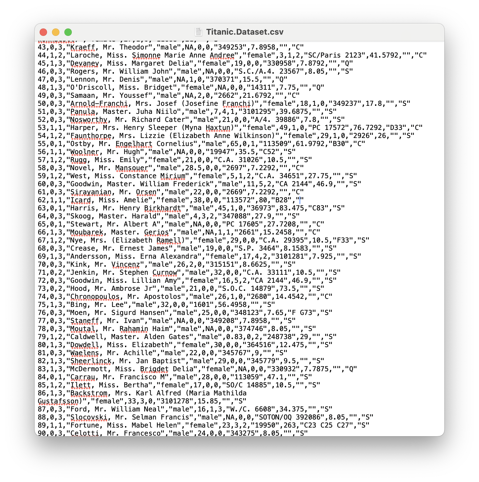
Figure 11.17: A Screenshot showing How to Clean up Titanic.Dataset

At this point, you can manually search for the missing values which we know appear on rows numbered 62 and 830. Above we see that the last entry on row 62 is "". We can now simply type in the value S into the space as shown below.

The blue line seen in the image above is the cursor.

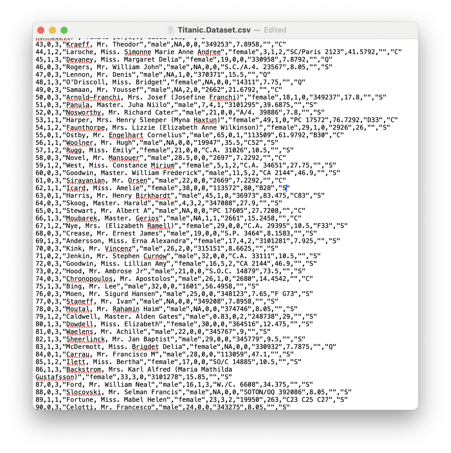
Figure 11.18: A Screenshot showing How to Clean up Titanic.Dataset

Scrolling further down shows that the last entry on row 830 is also "" as seen above and we can enter S here as well as shown below.

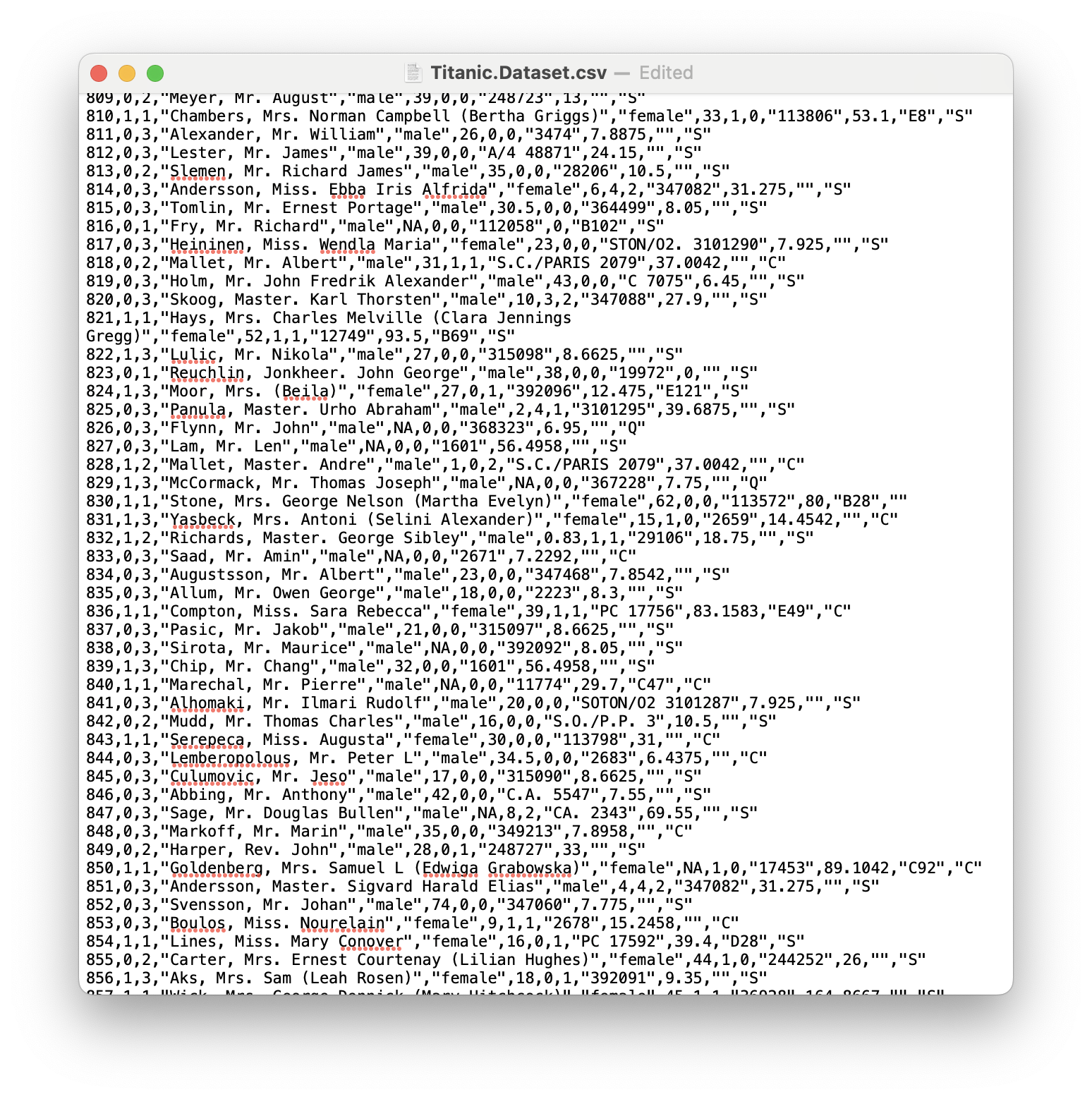
Figure 11.19: A Screenshot showing How to Clean up Titanic.Dataset

Saving the file should now give you an updated .csv file.

• Using a Spreadsheet Program: We now show how to handle this in a spreadsheet program. We will show it being done in Google Sheets, but the process should be nearly identical in similar programs. We begin by loading the file as shown below.

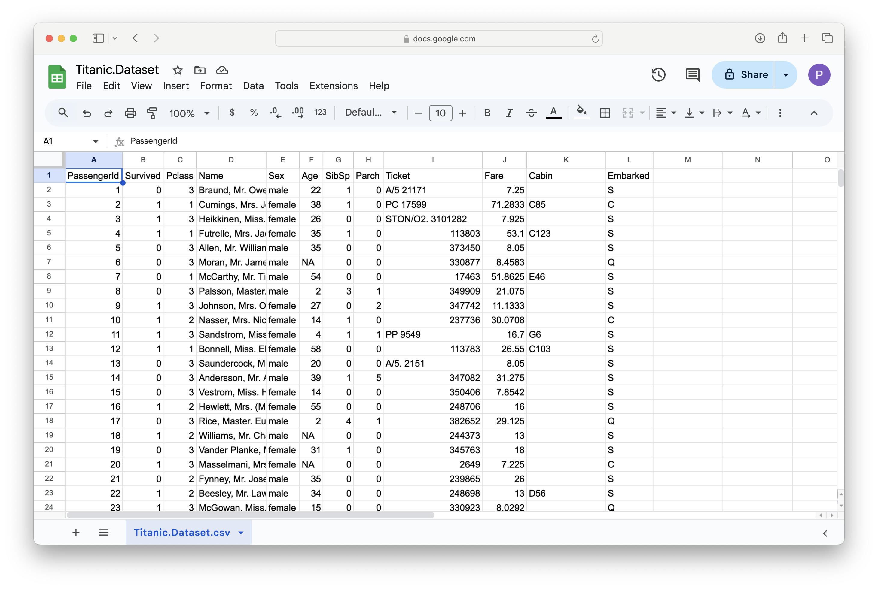
Figure 11.20: A Screenshot showing How to Clean up Titanic.Dataset

We can then scroll to find a blank entry in the Embarked column as shown below.

Figure 11.21: A Screenshot showing How to Clean up Titanic.Dataset

We can then type in the value of S into the missing cell.

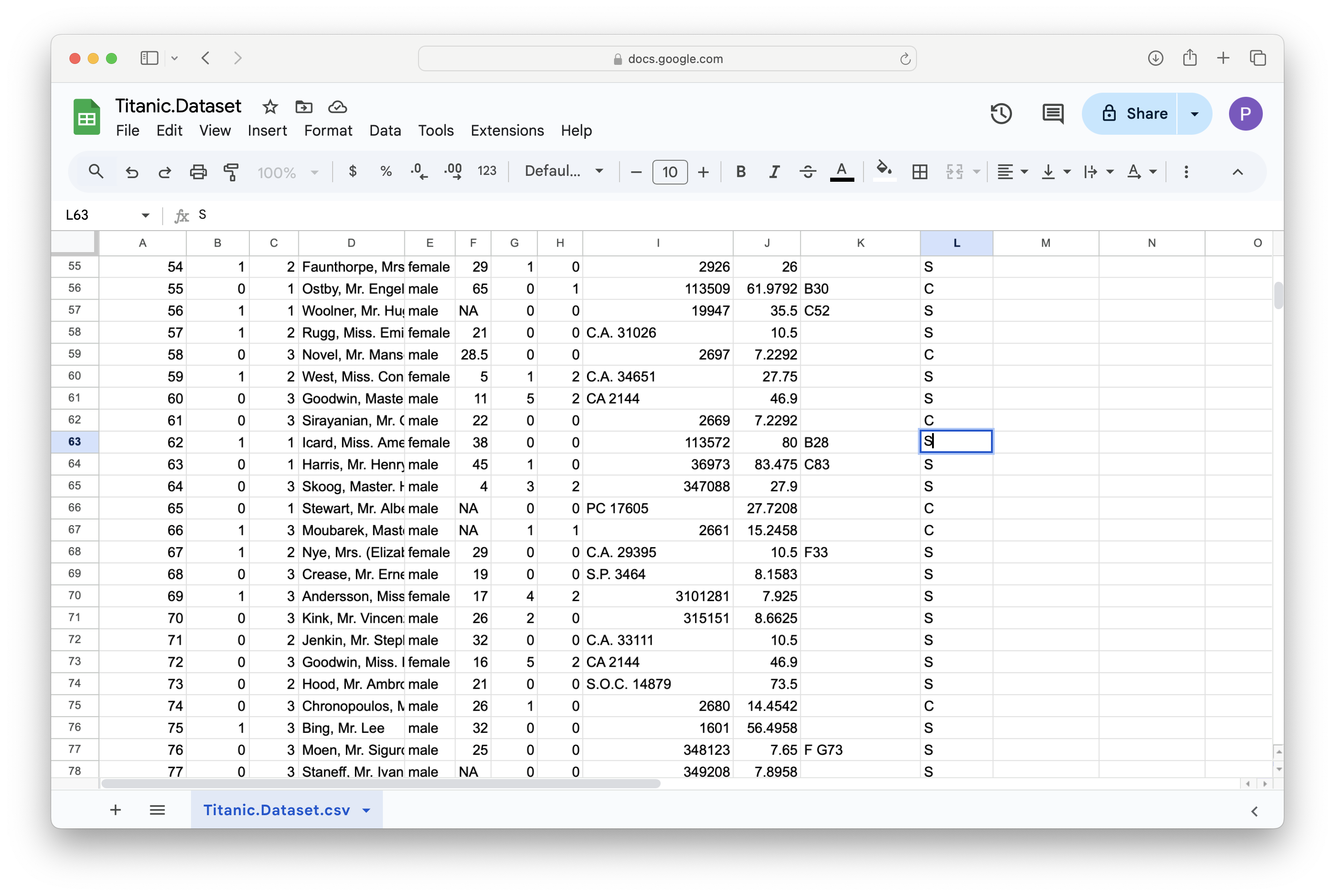
Figure 11.22: A Screenshot showing How to Clean up Titanic.Dataset

We can repeat this process for row 830 as shown in the next two images.

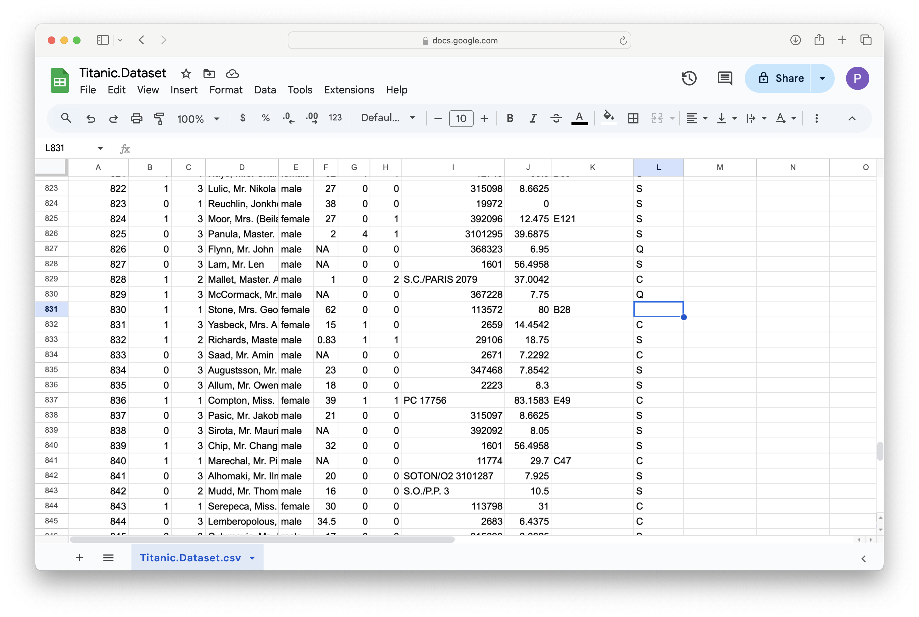
Figure 11.23: A Screenshot showing How to Clean up Titanic.Dataset

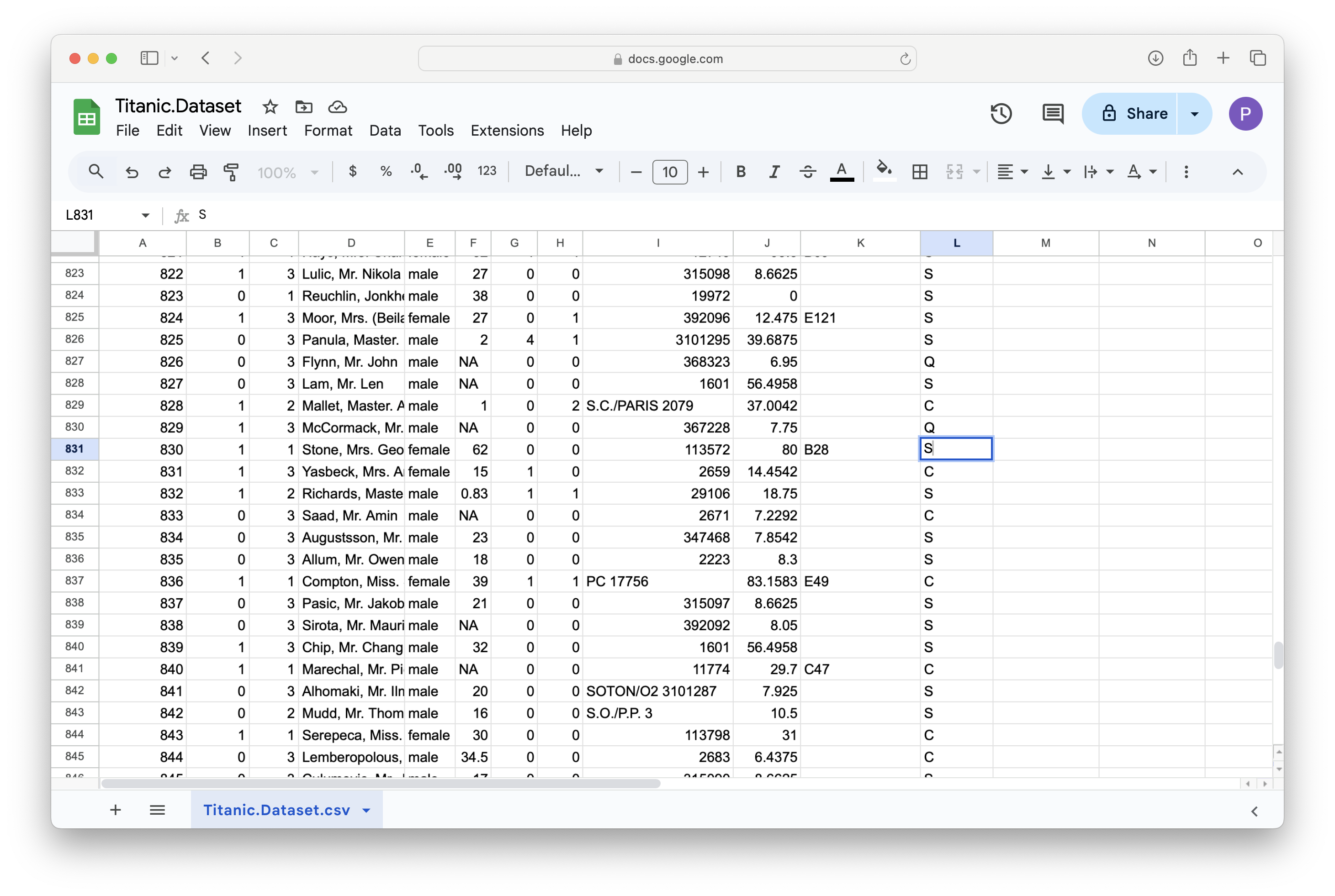
Figure 11.24: A Screenshot showing How to Clean up Titanic.Dataset

Then, at least in Google Sheets, you go to File > Download and select Comma Separated Values.

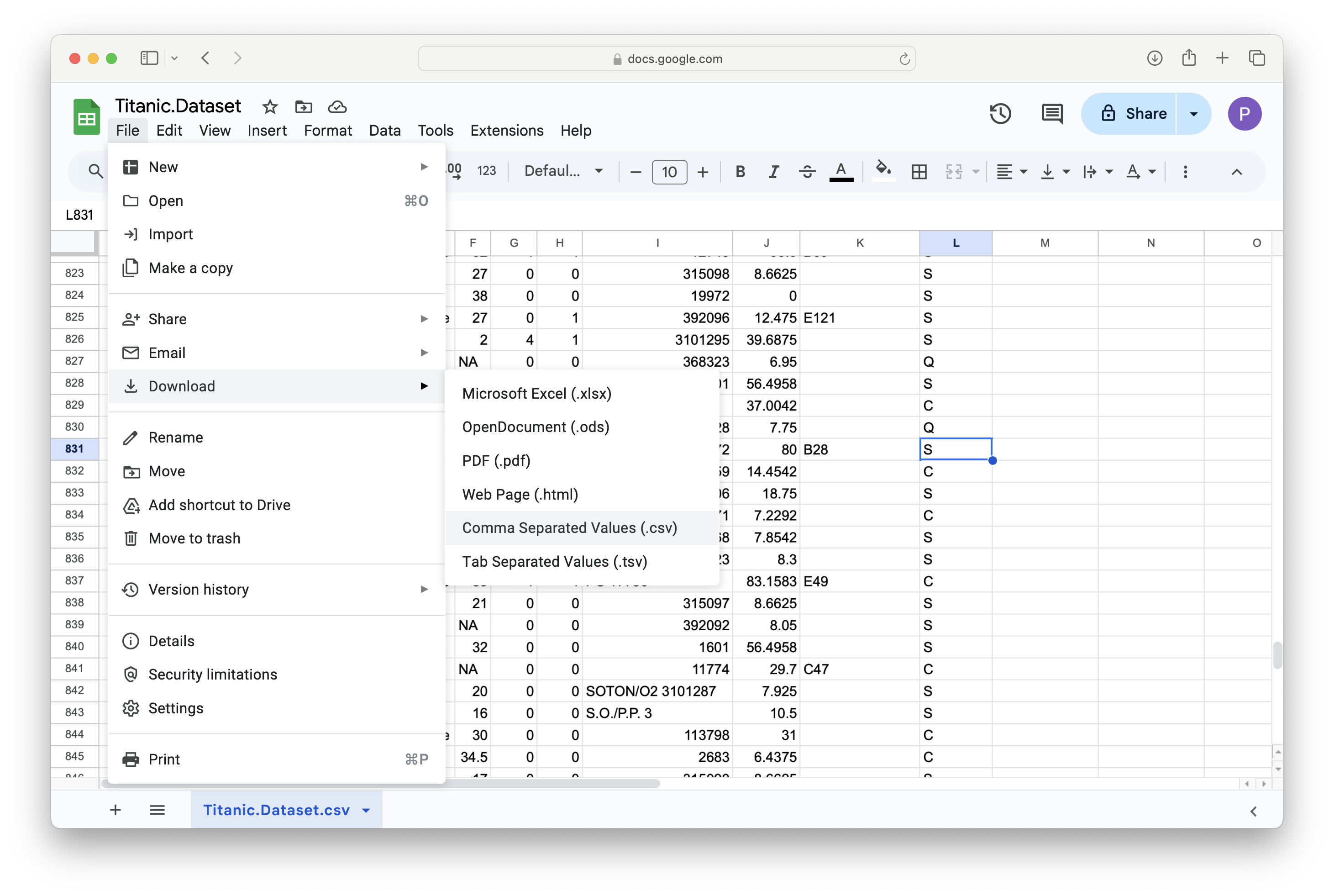
Figure 11.25: A Screenshot showing How to Clean up Titanic.Dataset

The updated file should now be on your computer.

• Importing to RStudio: Finally, we show how to get the .csv file back into RStudio. We begin by going to the upper right pane and clicking on Environment and then Import Dataset and finally selecting From Text (base)....

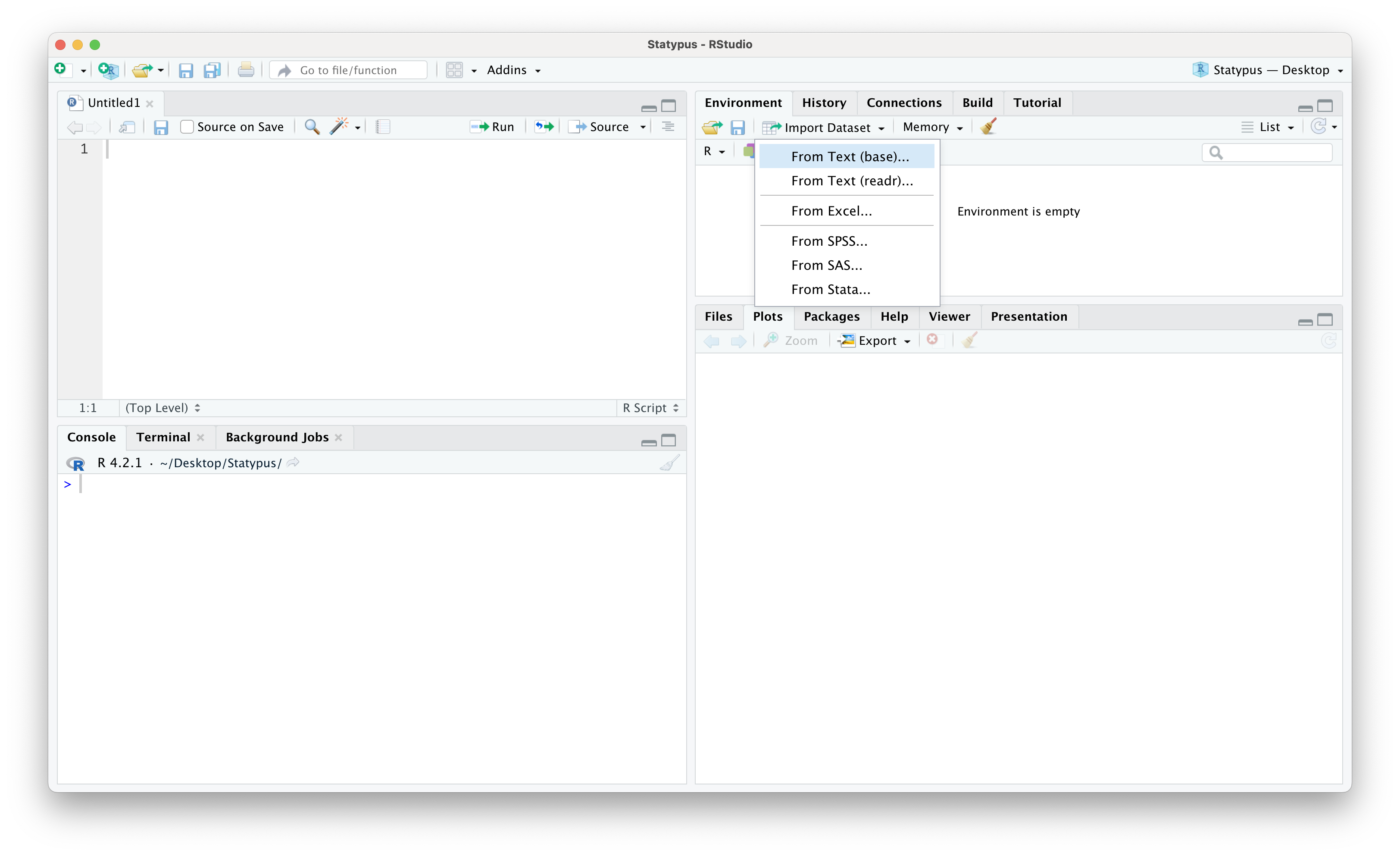
Figure 11.26: A Screenshot showing How to Clean up Titanic.Dataset

This should bring up a window on your computer to find the file created in one of the ways above. At this point, make sure that you select Yes for Heading and set Name to what you want the updated version to be.

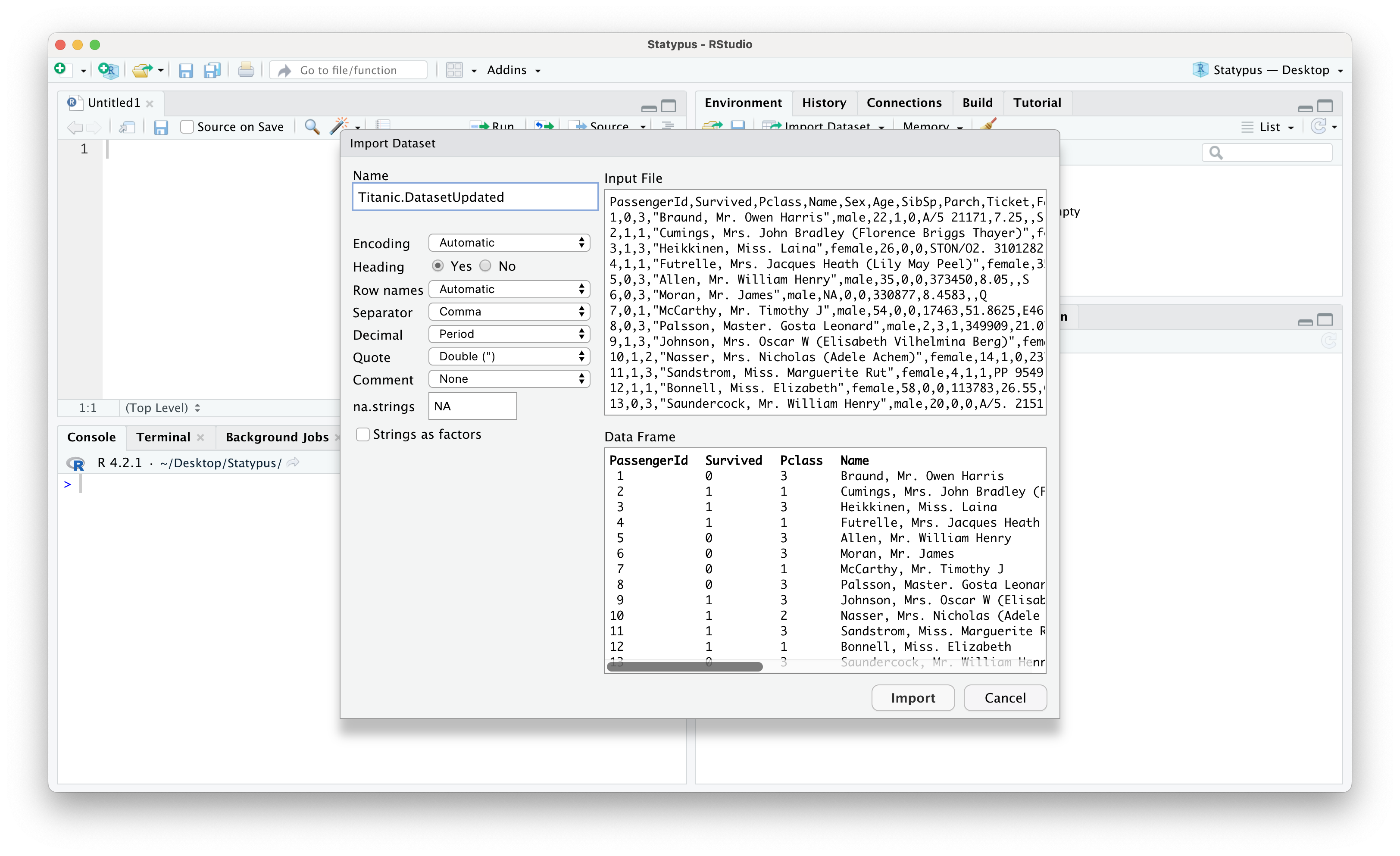
Figure 11.27: A Screenshot showing How to Clean up Titanic.Dataset

Below we see the result of having set the name to Titanic.DatasetUpdated as well as the result of running table on this new dataset to see that we no longer have any blank values.

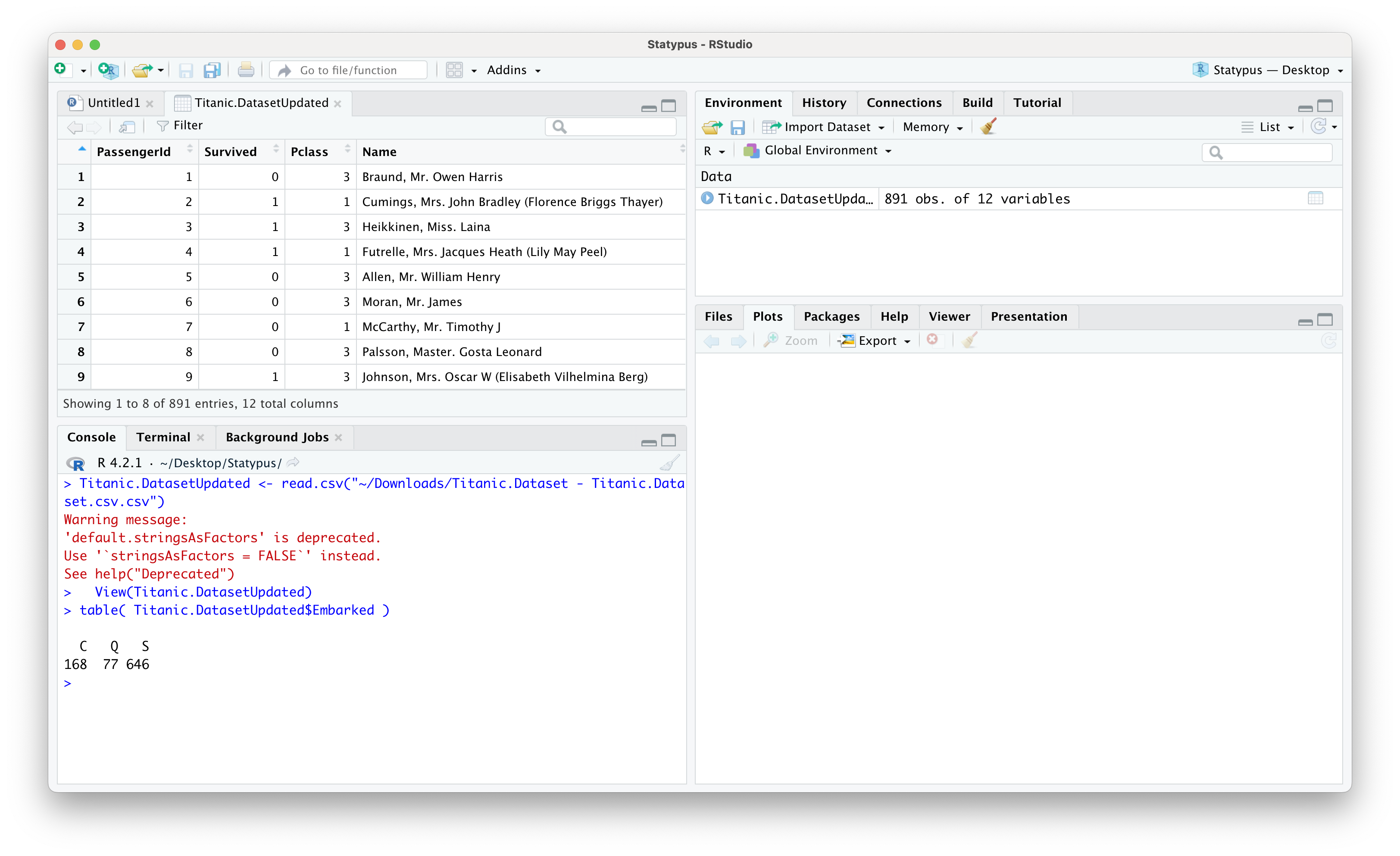
Figure 11.28: A Screenshot showing How to Clean up Titanic.Dataset

• Using Some R Ninjutsu: There are ways to make the update within RStudio, but we will not go into depth here. We simply offer a code chunk that would create a copy of Titanic.Dataset known as dd (so that we do not modify the original file, but only a copy), then updates the values using the middle line, and finally makes a copy of the updated file with the user friendly name, Titanic.Dataset.Updated.

dd <- Titanic.Dataset
dd$Embarked[ dd$PassengerId %in% c( 62, 830 ) ] <- "S"
Titanic.Dataset.Updated <- dd

---

180. Fauna of Australia. Vol. 1b. Australian Biological Resources Study (ABRS)↩︎

181. The term “chi square” is actually more common than “chi squared” in many introductory statistics books. There are reasons for this awkward terminology which can be investigated on math.stackexchange.com. However, we will adopt the convention of calling it “chi squared” to match the terminology of R.↩︎

182. It is possible to also look at the distribution of sample standard deviation, but it turns out that while the sample variance is an unbiased estimator of the population variance, the same is not true if we look at the standard deviation. The curious reader is encouraged to investigate such resources as section 5.6 of the book published at probstatsdata.com.↩︎

183. See the Appendix section entitled Alternate CLT for a discussion on how this compares to choices made in the Central Limit Theorem.↩︎

184. In fact, the \(\chi^2\) distribution with \(n\) degrees of freedom is defined off the square of \(n\) independent \(z\) or Standard Normal variables. Using the sample mean, \(\bar{x}\), in the calculations of the deviations is what reduces the degrees of freedom because the last deviation is not independent. I.e. if we know any \(n-1\) of the deviations, then we know the last deviation. In general, the degrees of freedom is the smallest number of deviations we must have to definitely know all of them. This will come into play when we look at the use of \(\chi^2\) in testing for the independence of categorical data.↩︎

185. See this article for more information.↩︎

186. To keep the flow of our analysis going, we won’t go into much detail about round here. You are encouraged to look at ?round if you want more information.↩︎

187. Please refer to Chapter 7 for a more precise explanation of what \(p\)-value measures.↩︎

188. The value in test$residuals is actually (Observed - Expected)/\(\sqrt{\text{Expected}}\) which can be useful as it does show which observed values are less than their expected values. However, this information is not directly necessary for the calculation of \(X^2\), so we simply report test$residuals^2.↩︎

189. We won’t get into the technicalities of this on Statypus, but the curious reader can see Wikipedia or a higher level textbook.↩︎

190. This is exactly why we used the t() function when we created columns.↩︎

191. It is worth noting that the last row and column values here are the opposites of the actual deviations shown above except for the cell which is in both the removed row and column which is exactly the same as the actual deviation.↩︎

192. The \(\chi^2\) test also should only be applied when each expected cell is at least 5.↩︎

193. The passengers name was Mrs.Martha Evelyn Stone, but her reservation was made under the name “Stone, Mrs. George Nelson (Martha Evelyn).” This indicates that Martha was forced to purchase her ticket under her husband’s name with her name as a parenthetical comment.↩︎