Chapter 13 Other Distributions and Simulations

Figure 13.1: A Statypus Professor Giving a Lecture

Platypuses have two layers of fur. The second layer serves as a sort of “dry suit” allowing it to trap a layer of air near its skin which insulates it and also allows it to remain buoyant.²⁰⁸

This Chapter has yet to be written. Please reach out to the author if you have any immediate questions.

FILL INTRODUCTION

New R Functions Used

All functions listed below have a help file built into RStudio. Most of these functions have options which are not fully covered or not mentioned in this chapter. To access more information about other functionality and uses for these functions, use the ? command. E.g. To see the help file for replicate, you can run ?replicate or ?replicate() in either an R Script or in your Console.

We will see the following functions in Chapter 13.

dgeom(): Density function for the geometric distribution.
pgeom(): Distribution function for the geometric distribution.
qgeom(): Quantile function for the geometric distribution.
rgeom(): Random number generation for the geometric distribution.
ppois(): Distribution function for the Poisson distribution.
qpois(): Quantile function for the Poisson distribution.
rpois(): Random number generation for the Poisson distribution.
replicate(): Allows for repeated evaluation of an expression (which will usually involve random number generation).
anyDuplicated(): Determines which elements of a vector or data frame are duplicates of elements with smaller subscripts.
cumsum(): Returns a vector whose elements are the cumulative sums of the elements of the argument.
rle(): Run Length Encoding: Computes the lengths and values of runs of equal values in a vector.

The functions cumsum() and rle() are only used in the challenging bonus problems and do not have any explanation here. Use ?cumsum or ?rle in your RStudio Console for help with these.

13.1 The Geometric Distribution

The Geometric distribution is used when we are interested in the number of failures that occur before the first success in a series of independent Bernoulli trials. While the Binomial distribution (Chapter 8) asks “How many successes do I get in \(n\) trials?”, the Geometric distribution asks “How many times do I fail before I finally succeed?”

In R’s implementation of the geometric functions, the random variable \(X\) represents the number of failures before the first success. This is an important distinction, as some textbooks count the total number of trials instead.

13.1.1 The Geometric Density Function

The dgeom() function calculates the probability mass function (PMF).

The syntax of dgeom() is:

dgeom( x, prob )

where the arguments are:

x: The number of failures before the first success.
prob: The probability of success on each trial.

Suppose a student is guessing on a multiple-choice quiz where each question has 4 options (\(p = 0.25\)). What is the probability that they get their first correct answer on the 4th question? This means they had exactly 3 failures before their first success.

dgeom( x = 3, prob = 0.25 )

## [1] 0.1054688

13.1.2 The Geometric Distribution Function

If we want to find the probability of a range of outcomes—such as the probability of succeeding within a certain number of attempts—we use the cumulative distribution function, pgeom().

The syntax of pgeom() is:

pgeom( q, prob, lower.tail = TRUE )

where the arguments are:

q: The number of failures.
prob: The probability of success.
lower.tail: If TRUE, it calculates \(P(X \leq q)\), otherwise \(P(X > q)\).

For our quiz-taker, the probability that they get their first right answer within the first 5 questions (meaning 4 or fewer failures) would be:

pgeom( q = 4, prob = 0.25, lower.tail = TRUE )

## [1] 0.7626953

13.1.3 The Geometric Quantile Function

The syntax of qgeom() is

qgeom( p, prob, lower.tail )     #This code will not run unless the necessary values are inputted.

where the arguments are:

x: Quantity to be evaluated for
prob: Probability of success on each trial.
lower.tail: If TRUE, the result is q such that \({\text{p} = P(X \leq \text{q} )}\) and if FALSE, the result is q such that \({\text{p} = P(X > \text{q})}\). lower.tail is set to TRUE by default.

13.1.4 The Geometric Random Function

The syntax of rgeom() is

rgeom(n, prob)     #This code will not run unless the necessary values are inputted.

where the arguments are:

n: Number of observations.
prob: Probability of success on each trial.

Example 13.1 Three way tool finally right

Socks <- rgeom(100,1/3)
head(Socks)

## [1] 0 0 2 3 3 1

table(Socks)

## Socks
##  0  1  2  3  4  5  6  8  9 10 11 18 
## 31 23 17  9  4  5  4  2  1  1  2  1

Example 13.2 Number of heads before first tails

set.seed(03271985)
FirstT <- rgeom(100,1/2)
table(FirstT)

## FirstT
##  0  1  2  3  4  5  6 13 
## 47 24 13  8  4  2  1  1

Example 13.3 First time rolling a 7²⁰⁹

rgeom(100,1/6)

##   [1]  1  0  4  2  3  4  2 11  2 14 23  4  5  2 12  4  6  4  1  3  1  3  0  0 12
##  [26]  9  4  0  1  7  1 11  1  5  3  0  2  1  2  0  1  1 12  5  1  6  6  3 17  4
##  [51]  0  0  0  7  9 15  2  4  4  3  3  1  2  2  0  6  1  2  2  8 16  5  1  4  2
##  [76]  0  8  9  3  0 10 20  1  1  8  1  2  3  3  0  5  0 13  2  0  1  2  6  3  7

13.1.5 The Shape of the Geometric Distribution

Later in this chapter, we will run complex simulations, but it is helpful to see what distributions look like. We can use the random generation functions to “observe” thousands of trials at once. The Geometric distribution is always right-skewed because it is more likely to succeed early than to suffer a massive string of failures.

bin_width = 1
data <- rgeom( n = 100000, prob = 0.1 )
hist( data, 
      freq = TRUE, 
      breaks = seq( 
                      from = min( data, na.rm = TRUE ) - 0.5, 
                      to = max( data, na.rm = TRUE ) + bin_width - 0.5, 
                      by = bin_width
                  )
    )

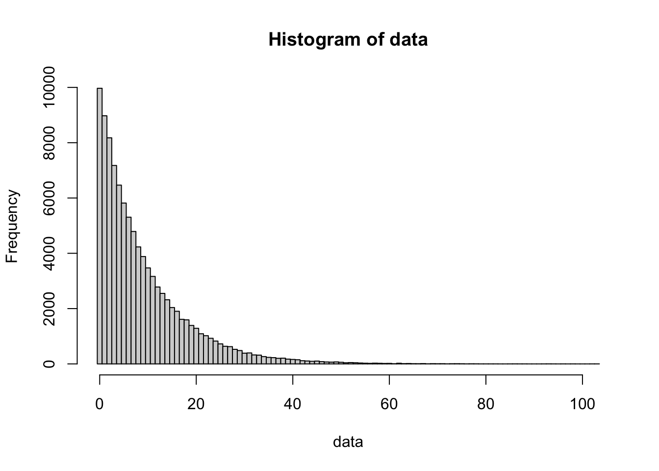
Figure 13.2: 100,000 simulations of a Geometric process (p=0.1)

bin_width = 1
data <- rgeom( n = 100000, prob = 0.2 )
hist( data, 
      freq = TRUE, 
      breaks = seq( 
                      from = min( data, na.rm = TRUE ) - 0.5, 
                      to = max( data, na.rm = TRUE ) + bin_width - 0.5, 
                      by = bin_width
                  )
    )

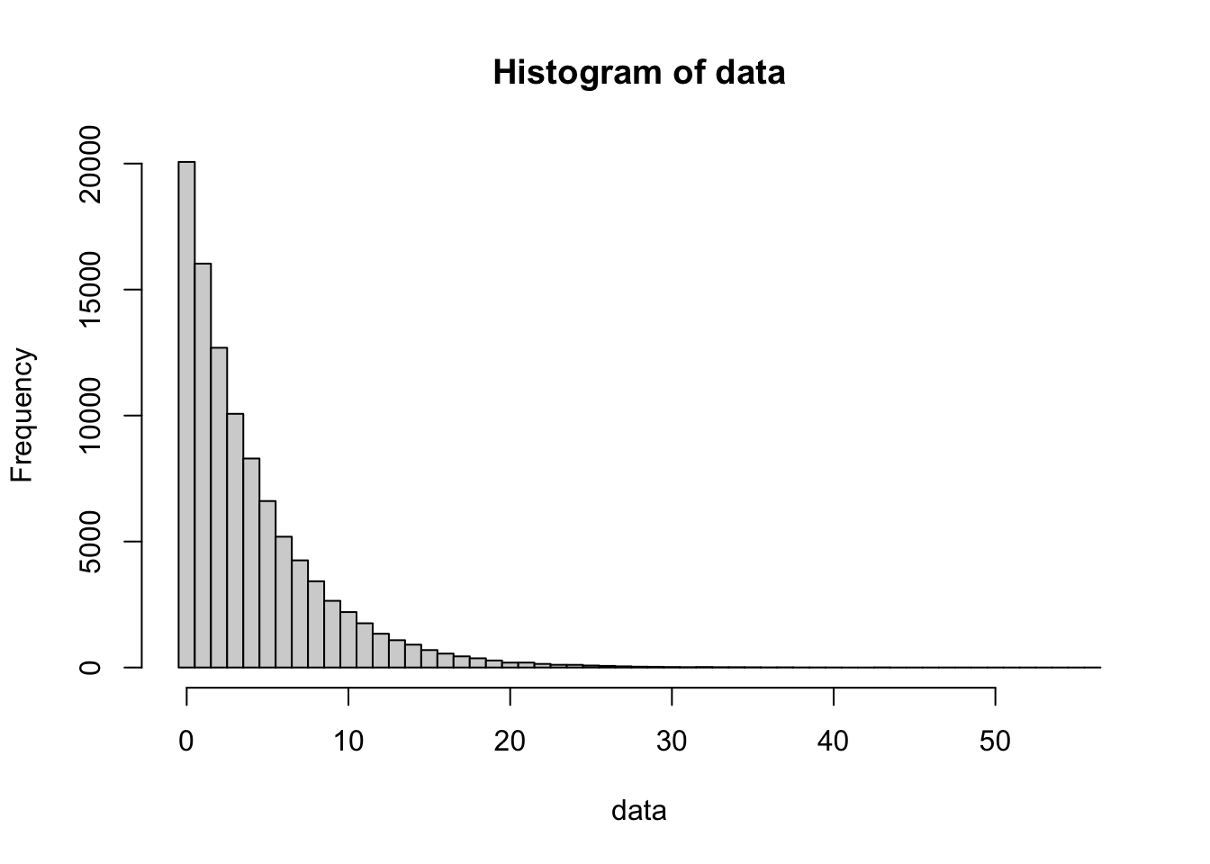
Figure 13.3: 100,000 simulations of a Geometric process (p=0.2)

bin_width = 1
data <- rgeom( n = 100000, prob = 0.5 )
hist( data, 
      freq = TRUE, 
      breaks = seq( 
                      from = min( data, na.rm = TRUE ) - 0.5, 
                      to = max( data, na.rm = TRUE ) + bin_width - 0.5, 
                      by = bin_width
                  )
    )

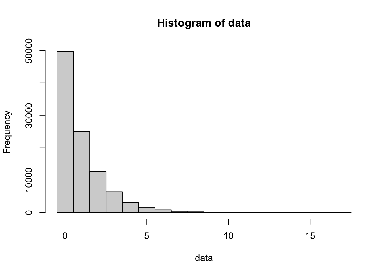
Figure 13.4: 100,000 simulations of a Geometric process (p=0.5)

bin_width = 1
data <- rgeom( n = 100000, prob = 0.8 )
hist( data, 
      freq = TRUE, 
      breaks = seq( 
                      from = min( data, na.rm = TRUE ) - 0.5, 
                      to = max( data, na.rm = TRUE ) + bin_width - 0.5, 
                      by = bin_width
                  )
    )

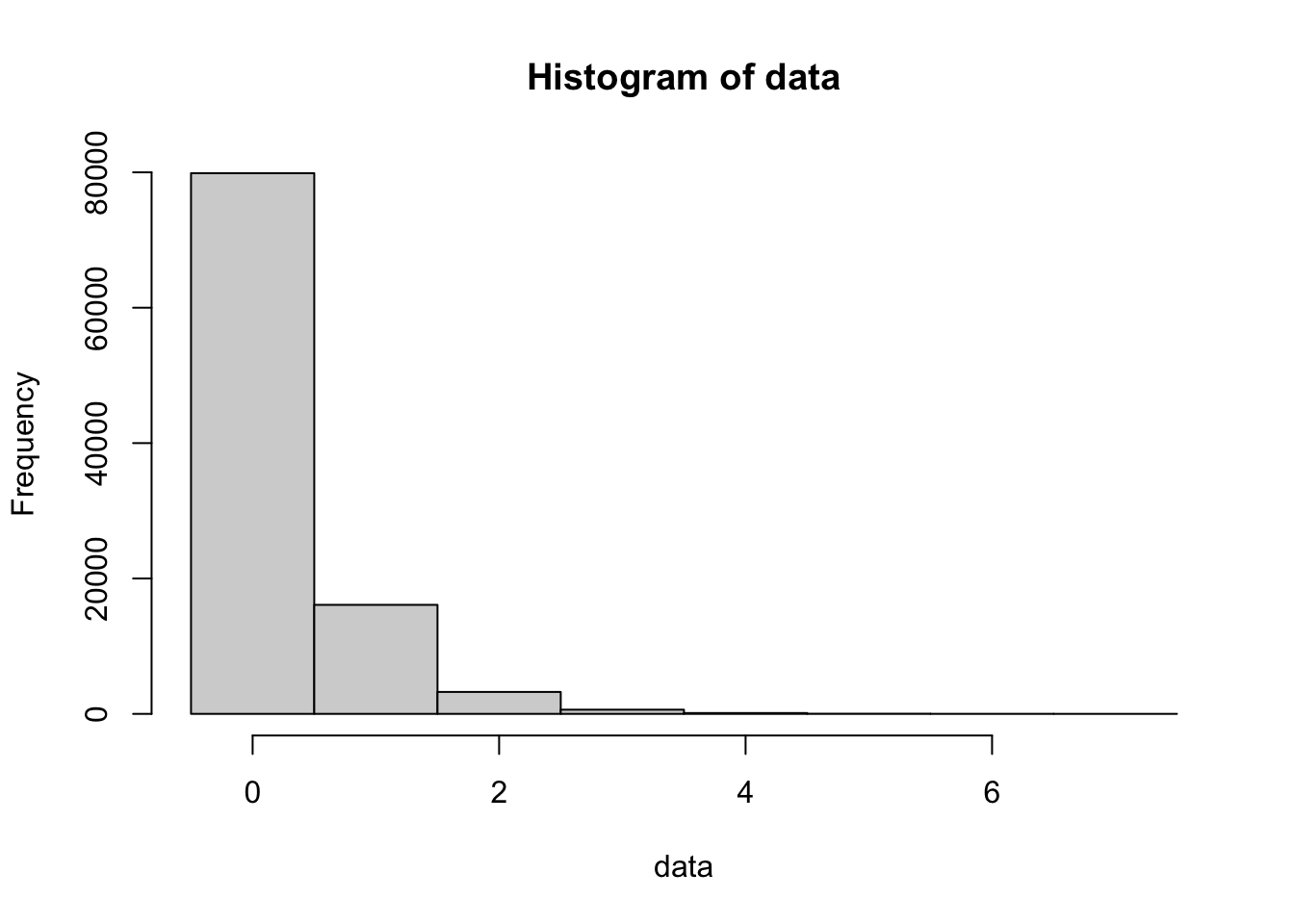
Figure 13.5: 100,000 simulations of a Geometric process (p=0.8)

13.2 The Poisson Distribution

The Poisson distribution is a discrete probability distribution used to model the number of events occurring within a fixed interval of time or space. While the Binomial distribution deals with a set number of trials, the Poisson distribution deals with a rate of occurrence (often denoted by the Greek letter lambda, \(\lambda\)).

Common examples include

The number of emails received in an hour.

The number of mutations in a specific stretch of DNA.

The number of platypuses spotted along a 1-kilometer stretch of a river.

13.2.1 The Poisson Density Function

The dpois function calculates the probability of seeing exactly x events in a given interval.

The syntax of dpois() is:

dpois( x , lambda )

where the arguments are:

x: The number of failures.
lambda: The average rate (\(\lambda\)).

Suppose a specific stretch of river averages 3 platypus sightings per day, that is \(\lambda = 3\). What is the probability of seeing exactly 2 platypuses today?

dpois( x = 2, lambda = 3 )

## [1] 0.2240418

13.2.2 The Poisson Distribution Function

To find the probability of a cumulative number of events (e.g., at most or more than), we use ppois.

The syntax of ppois() is:

ppois( q, lambda, lower.tail = TRUE )

where the arguments are: * q: The number of events (quantile). * lambda: The average rate (\(\lambda\)). * lower.tail: If TRUE (default), calculates P(X <= q). If FALSE, calculates P(X > q).

If the average number of customer complaints at a watch repair shop is 1.5 per week, what is the probability that they receive more than 3 complaints in a single week?

ppois( q = 3, lambda = 1.5, lower.tail = FALSE )

## [1] 0.06564245

13.2.3 The Poisson Quantile Function

The syntax of qpois() is

qpois( p, lambda, lower.tail )     #This code will not run unless the necessary values are inputted.

where the arguments are:

x: Quantity to be evaluated for
lambda: The average rate (\(\lambda\)).
lower.tail: If TRUE, the result is q such that \({\text{p} = P(X \leq \text{q} )}\) and if FALSE, the result is q such that \({\text{p} = P(X > \text{q})}\). lower.tail is set to TRUE by default.

13.2.4 The Poisson Random Function

The syntax of rpois() is

rpois( n, lambda )     #This code will not run unless the necessary values are inputted.

where the arguments are:

n: Number of observations.
lambda: The average rate (\(\lambda\)).

13.3 Simulations

This section uses simulation as the center of a study of probability. Simulations can allow a study of probability questions that are not easily answered with abstract techniques. Simulation also plays a fundamental role in modern statistical methods such as resampling, bootstrapping, non-parametric statistics, and genetic algorithms.

We first used the R function sample() when finding a SRS in Chapter 2, but we now wish to leverage the function even further.

Rewrite the following For an experiment with a finite sample space \(S =\{x_1, x_2, \ldots, x_n\}\), sample() can simulate one or many trials of the experiment. Essentially, sample treats \(S\) as a bag of outcomes, reaches into the bag, and picks one.

Sample() already dealt with in Chapters 2, 3, and 6

The syntax of sample is

sample( x , size , replace , prob )

where the arguments are:

x: The vector of elements from which you are sampling.
size: The number of samples you wish to take.
replace: Whether you are sampling with replacement or not. Sampling without replacement means that sample will not pick the same value twice, and this is the default behavior. Pass replace = TRUE to sample if you wish to sample with replacement.
prob: A vector of probabilities or weights associated with x. It should be a vector of non-negative numbers of the same length as x.

If the sum of prob is not 1, it will be normalized. That is, each value in prob will be taken to be out of the sum of prob. For example, if the values in prob were 0.2, 0.3, and 0.4, then the actual probabilities would be 0.2/0.9 = 2/9, 0.3/0.9 = 1/3, and 0.4/0.9 = 4/9. If prob is not provided, then each element of x is considered to be equally likely.

replicate(n , expr)

repeats the expression stored in expr a series of n times and stores the resulting values as a vector.

For complicated simulations, we strongly recommend that you follow the workflow as presented above; namely,

Write repeatable code that performs the experiment a single time.
Replicate the experiment a small number of times and check the results.

replicate( 100 , { 
      EXPERIMENT GOES HERE    
      } )

Replicate the experiment a large number of times and store the result.

event <- replicate( 10000 , { 
                      EXPERIMENT GOES HERE 
                      } )

Finally, estimate the probability using mean.

mean( event )

It is much easier to trouble-shoot your code this way, as you can test each line of your simulation separately.

Example 13.4 (First Look at M and Ms) According to Rick Wicklin²¹⁰, the proportion of M&M’s of various colors produced in the New Jersey M&M factory are as shown in the table below.

M&M Candies, Photo by [Evan Amos](https://commons.wikimedia.org/wiki/File:Plain-M&Ms-Pile.jpg)

Figure 13.6: M&M Candies, Photo by Evan Amos

\[\begin{array}{|l|c|} \hline \text{Color} & \text{Percentage}\\ \hline \text{Blue} & 25.0\\ \text{Orange} & 25.0\\ \text{Green} & 12.5\\ \text{Yellow} & 12.5\\ \text{Red} & 12.5\\ \text{Brown} & 12.5\\ \hline \end{array}\]

mm.colors <- c( "Blue", "Orange", "Green", "Yellow", "Red", "Brown" )
mm.probs <- c( 25, 25, 12.5, 12.5, 12.5, 12.5 )
bag <- sample(
  x = mm.colors,
  size = 35,
  replace = TRUE,
  prob = mm.probs
)
sum( bag == "Blue" ) # counts the number of Blue M&M's

## [1] 8

Exercises

Exercise 13.1 A certain mechanical watch movement has a 1 in 500 chance of having a specific assembly defect. If a watchmaker examines movements one by one, what is the probability that they find the first defect on exactly the 100th movement? (Hint: How many failures occur before that 100th movement?)

Exercise 13.2 A vintage watch collector finds that, on average, a rare timepiece appears on a specific auction site 0.8 times per month. What is the probability that at least one such watch appears next month?

Exercise 13.3 Find the “odds” of Patricia Demauro’s accomplishment.

Exercise 13.4 Assume we roll a standard 6 sided die and a fair 12 sided die. Estimate the probability that the value on the 6 sided die is greater than that on the 12 sided one.

Exercise 13.5 Estimate the probability that the sum on two dice is greater than the sum on three dice.

Exercise 13.6 Watch the video below and show via simulation that the dice ranking shown in the video is correct.

Challenge Problems:

Exercise 13.7 Estimate the probability of having at least 6 successive Heads or Tails if you flipped a coin 100 times. What about 7 successive tosses of Heads or Tails? [Hint: Look up rle() in RStudio.]

Exercise 13.8 Refer to https://en.wikipedia.org/wiki/Craps#Pass_line and estimate the probability of winning a Pass line bet. [Warning: This will require more functions than given here.]

[Warning: The following problem(s) are even harder and will likely require a “loop” of some sort.]

“Platypus facts file”. Australian Platypus Conservancy.↩︎
See https://casino.betmgm.com/en/blog/luckiest-craps-players-in-the-world/ for more information.↩︎
C Purtill, “A Statistician Got Curious about M&M Colors and Went on an Endearingly Geeky Quest for Answers,” Quartz, March 15, 2017, https://qz.com/918008/the-color-distribution-of-mms-as-determined-by-a-phd-in-statistics/.↩︎